
MATLAB Scripting API
Introduction
This document describes Audio Weaver’s MATLAB automation API. It allows you to leverage the power of MATLAB to configure and control Audio Weaver. The API can be used for parameter calculation, visualization, general automation, regression tests, and even full system building. The API is an advanced feature and assumes that the user is familiar with MATLAB.
The most straightforward use of the API allows MATLAB to interact with the Audio Weaver Designer GUI. This is documented in Interacting with Audio Weaver Designer and is sufficient for most users. More advanced scripting features are described in later sections.
MATLAB is an interpreted scripting language and all of the commands shown in this section can be typed in directly into MATLAB, or copy and pasted directly from this User's Guide.
Requirements
The API is compatible with MATLAB version 2017b or later. You’ll need a standard MATLAB license and the Signal Processing Toolbox. 32-bit and 64-bit versions of MATLAB are supported.
The MATLAB API is included with the “Pro” versions of Audio Weaver; it is not part of the Standard version.
Setup
After installing Audio Weaver Developer or Pro, update MATLAB's search path to include the directory:
<AWE>\matlab
where <AWE> represents the installation directory. This directory contains the primary set of MATLAB scripts used by the tool. Note that you only have to add a single directory to the MATLAB path and not all of the subdirectories recursively. The MAT
LAB menu item "File -> Setup Path…" can be used to update the path. Once the path is set, issue the command:
awe_designer
This launches the Audio Weaver Server followed by the Designer application. It also configures additional directories, and initializes global variables. If you just want to launch the Server and configure MATLAB to run scripts, then simply execute:
awe_init
If you accidentally shut down the Server while using Audio Weaver Designer, then press the Reconnect to Server button found on the toolbar.

If you are not using Designer, then you can reconnect to the Server by reissuing the awe_init command.
If you forget to rerun awe_init.m, you'll get an error similar to the one shown below next time MATLAB tries to communicate with the Server:
??? Error using ==> awe_server_command at 47
Server Command Failure:
       Command sent to server:  "get_target_info"
       Server response:  "failed, transmit error 0xffffffff"

Error in ==> target_get_info at 89
    str=awe_server_command('get_target_info');
Audio Weaver supports multiple simultaneous installations. Install each version in a separate directory. Then, select the version to use by configuring the MATLAB path to point to the appropriate <AWE>\matlab directory and then run the associated awe_init.m script. You can check which version of Audio Weaver is active by the command
>> awe_version

Audioweaver Version Number:
    awe server:          32568
    awe_module:          32465
    awe_subsystem:       32465
    awe_variable:        31481
    pin:                 32555
    pin_type:            32495
    feedback_pin_type:   31604
    connection:          30792
Online Help
All of the Audio Weaver MATLAB functions have usage instructions within the function header. To get help on a particular function, type
help function_name
Additional help is available for audio modules. The command
awe_help
creates a list of available audio modules in the MATLAB command window. A partial list is shown below:
>> awe_help
GPIO_module - Misc
abs_fract32_module - BasicAudioFract32
abs_module - BasicAudioFloat32
acos_module - MathFloat32
adder_fract32_module - BasicAudioFract32
adder_int_module - BasicInt32
adder_module - BasicAudioFloat32
agc_attack_release_fract32_module - BasicAudioFract32
Each of the modules appears as a hyperlink, and clicking on an item provides detailed module specific help. The help provided is above and beyond the comments shown in the file header and accessed via the standard MATLAB “help” command. You can also obtain help for a specific module using the MATLAB command line. For example, to get help on the FIR filter module, type:
awe_help fir_module
The help documentation is provided in HTML format.
Interacting with Audio Weaver Designer
The most basic way of using the MATLAB API is to get and set parameters in a system that is loaded in Audio Weaver Designer.
Manipulating Parameters
Assume that you have the system “Example1.awd” open in Designer.
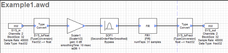
Then from the MATLAB prompt, type
GSYS = get_gsys('Example1.awd');
This returns a MATLAB data structure which contains the entire state of the Designer GUI. We won’t go into the details here; the only item of interest is the field .SYS which we call the system structure
GSYS.SYS

 = NewClass // Newly created subsystem

  SYS_toFloat: [TypeConversion]
      Scaler1: [ScalerV2]
         SOF1: [SecondOrderFilterSmoothed]
         FIR1: [FIR]
  SYS_toFract: [TypeConversion]
The system structure contains one entry per module in the system. Looking more closely at Scaler1 we see all of the internal parameters of the module:
GSYS.SYS.Scaler1

Scaler1 = ScalerV2 // General purpose scaler with a single gain

           gain: 0         [dB] // Gain in either linear or dB units.
  smoothingTime: 10        [msec] // Time constant of the smoothing process.
           isDB: 1          // Selects between linear (=0) and dB (=1) operation
The first line displays 3 items:
“Scaler1” – the name of the module within the system.
“ScalerV2” – the underlying class name or type of the module.
“General purpose scaler …” – this is a short description of the function of the module.
The next three lines list exposed interface variables that the module contains. A variable may display applicable units in brackets (e.g, [msec]) and have a short description.
To change the gain of the module, type
GSYS.SYS.Scaler1.gain = -6;
The gain change occurs locally in the MATLAB environment; the system in Designer is unchanged. To send the updated system back to Designer, type
set_gsys(GSYS, 'Example1.awd');
If the system in Designer is built and running, then the gain change will also occur on the target processor when the command
GSYS.SYS.Scaler1.gain = -6;
is issued. The system in Designer doesn’t have the new gain value but the target processor does. You have to keep this in mind. Changes made by MATLAB update the target processor directly when in tuning mode but don’t update the system in Designer until you issue set_gsys.m.
Commonly Used Commands
This section describes commonly used MATLAB commands. More details can be found in subsequent sections.
Showing Hidden Variables
By default, the MATLAB API does not show hidden variables (e.g., filter state variables). If you would like to make these visible, type
global AWE_INFO;
AWE_INFO.displayControl.showHidden = 1;
AWE_INFO is a global variable which controls various aspects of Audio Weaver. The standard view of the SecondOrderFilterSmoothed module is
GSYS.SYS.SOF1

SOF1 = SecondOrderFilterSmoothed // General 2nd order filter designer with smoothing

     filterType: 0          // Selects the type of filter that is implemented.
           freq: 250       [Hz] // Cutoff frequency of the filter, in Hz.
           gain: 0         [dB] // Amount of boost or cut to apply, in dB if applicable.
              Q: 1          // Specifies the Q of the filter, if applicable.
  smoothingTime: 10        [msec] // Time constant of the smoothing process.
And now with hidden variables shown
GSYS.SYS.SOF1

SOF1 = SecondOrderFilterSmoothed // General 2nd order filter designer with smoothing

      filterType: 0          // Selects the type of filter that is implemented.
            freq: 250       [Hz] // Cutoff frequency of the filter, in Hz.
            gain: 0         [dB] // Amount of boost or cut to apply, in dB if applicable.
               Q: 1          // Specifies the Q of the filter, if applicable.
   smoothingTime: 10        [msec] // Time constant of the smoothing process.
    updateActive: 1          // Specifies whether the filter coefficients are updating
              b0: 1          // Desired first numerator coefficient.
              b1: 0          // Desired second numerator coefficient.
              b2: 0          // Desired third numerator coefficient.
              a1: 0          // Desired second denominator coefficient.
              a2: 0          // Desired third denominator coefficient.
      current_b0: 1          // Instantaneous first numerator coefficient.
      current_b1: 0          // Instantaneous second numerator coefficient.
      current_b2: 0          // Instantaneous third numerator coefficient.
      current_a1: 0          // Instantaneous second denominator coefficient.
      current_a2: 0          // Instantaneous third denominator coefficient.
  smoothingCoeff: 0.064493   // Smoothing coefficient. This is computed based on the smoothingTime, sample rate, and block size of the module.
           state: [2x2 float] // State variables. 2 per channel.
You’ll now see derived variables and state variables which are normally hidden from view.
Building Systems
If the system in Audio Weaver Designer is in Design mode, you can build the system using
GSYS = get_gsys('Example1.awd');
GSYS.SYS = build(GSYS.SYS);
and then you can start real-time audio playback with
test_start_audio;
Loading and Saving Designs
Instead of loading the GSYS structure from Designer, you can load it directly from disk
GSYS = load_awd('Example1.awd');
Then when you are done making modifications, save it to disk
save_awd('Example1.awd', GSYS);
Variable Ranges
Audio Weaver variables can have range information associated with them. To view a variables range information, you can type
GSYS.SYS.Scaler1.gain.range

ans =

   -24    24
If you try and set a value outside of the allowable range then a warning will occur:
GSYS.SYS.Scaler1.gain = -40;
Warning: Assignment to variable gain is out of range. Value: -40.  Range: [-24:24]
> In awe_variable_subsasgn at 64
  In awe_module.subsasgn at 86
  In awe_module.subsasgn at 128
To change a variables range, simply update the .range field
GSYS.SYS.Scaler1.gain.range = [-50 0];
The Basics of the MATLAB API
This tutorial walks you through the process of creating modules and subsystems within the Audio Weaver environment. Many of the features of the tool are presented with an emphasis on using existing audio modules. Writing new low-level modules is outside the scope of this tutorial and is described separately in the Audio Weaver Module Developers Guide. The tutorial assumes some familiarity with MATLAB.
Simple Scaler System
This example walks you through the process of creating a simple system containing a gain control. It takes you from instantiation in MATLAB through building the system using dynamic instantiation and finally real-time tuning.
Creating an Audio Module Instance
We begin by creating a single instance of a smoothly varying scaler module. This module scales a signal by a specified gain. The module is “smoothly varying” which means that the gain can be updated discontinuously and that the module performs internal sample-by-sample smoothing to prevent audio clicks. At the MATLAB command line type:
M=scaler_smoothed_module('foo');
The module is created and assigned to the variable “M”. The module also has an internal name “foo” which will become important when the module is added to a system. The function “scaler_smoothed_module” is referred to as the “MATLAB constructor function” for this module. Examine the contents of the variable M by typing
M
at the MATLAB prompt. (This time we leave off the semicolon which causes MATLAB to display the result to the command line.) We see:
foo = ScalerSmoothed // Gain control with linear units and smoothing

           gain: 1         [linear] // Gain in linear units.
  smoothingTime: 10        [msec] // Time constant of the smoothing process.
The first line displays 3 items:
“foo” – the name of the module assigned when the module was created.
“ScalerSmoothed” – the underlying class name or type of the module. Modules of the same class share a common set of functions.
“Gain control with…” – this is a short description of the function of the module.
The next two lines list exposed interface variables that the module contains. A variable may display applicable units in brackets (e.g, [msec]) and have a short description.
The scaler_smoothed_module smoothly ramps the gain using a first order exponential smoother. The time constant of the smoothing operation is controlled by the variable "smoothingTime".
The module M is implemented using MATLAB’s object oriented programming techniques. The module corresponds to the class @awe_module. (This is not important to the novice user but for people familiar with MATLAB, it explains the underlying MATLAB implementation.)
You can treat the module M as if it were a standard MATLAB structure. You can get and set values using the “.” notation:
M.gain=0.5;
M.smoothingTime=M.smoothingTime*2;
We then find that M has the values:
           gain: 0.5    [linear] // Gain in linear units.
  smoothingTime: 20     [msec] // Time constant of the smoothing process.
Creating a Subsystem
Our next step will be to create a subsystem containing the ScalerSmoothed module. A subsystem is one or more audio modules together with I/O pins and a set of connections.
SYS=target_system('Test', 'System containing a scaler', 1);
The first argument is the class name of the subsystem and the second argument is a short description. The third argument specifies that the subsystem will be run in real-time. The subsystem is assigned to the variable SYS and we can examine the subsystem by typing “SYS at the MATLAB prompt:
>> SYS
= Test // System containing a scaler
This looks similar to an audio module except that it is missing variables and instance names.
Adding I/O Pins
A subsystem also has “pins” that pass signals in and out of the subsystem. Let’s add an input pin to the system:
add_pin(SYS, 'input', 'in', 'audio input', new_pin_type(2, 32, 48000, 'fract32'));
where
‘input’ – controls whether the pin is an ‘input’ or ‘output’ to the subsystem.
‘in’ – a name or label for the pin. Keep this short since it appears on signal diagrams.
‘audio input’ – a description of the function of the pin. This can be longer and appears in some of the automatically generated documentation.
new_pin_type(2, 32, 48000, 'fract32') – this specifies that the pin contains 2 interleaved channels, each with 32 samples, at 48 kHz, with 32-bit fractional data.
In the same manner, add an output pin:
add_pin(SYS, 'output', 'out', 'audio output', new_pin_type(2, 32, 48000, 'fract32'));
The astute MATLAB user will recognize that we are violating MATLAB’s basic method of updating arguments in the calling environment. The commands above modify the object SYS in the calling environment. Typically, to accomplish this, you need to request an output argument from the function as in:
SYS=add_pin(SYS, 'input', 'in', 'audio input', new_pin_type(2, 32, 48000, 'fract32'));
This is a valid statement within the Audio Weaver environment, but for the sake of simplicity, certain functions update variables directly in the calling environment. For example, the add_pin() function updates the argument SYS and thus the return argument may be omitted.
Adding Modules
Now add an instance of the ScalerSmoothed module to the subsystem:
add_module(SYS, scaler_smoothed_module('scale'));
The add_module function always takes a system as the first argument and a MATLAB @awe_module object as the second argument. In doing so, there is no need to assign the module to an intermediate MATLAB variable. Let’s look at SYS
>> SYS
 = Test // System containing a scaler

scale: [ScalerSmoothed]
We now see a module named “scale” of class “ScalerSmoothed” listed. Since a new instance of the ScalerSmoothed was created, it is initialized to its default values. We can see this by typing “SYS.scale” at the command line:
>> SYS.scale
scale = ScalerSmoothed // Gain control with linear units and smoothing

           gain: 1         [linear] // Gain in linear units.
smoothingTime: 10        [msec] // Time constant of the smoothing process.
Note that Audio Weaver represents subsystems and modules as structures within the MATLAB environment. You access internal modules using the “.” notation. You can also set variables directly as:
SYS.scale.gain=0.5;
SYS.scale.smoothingTime=SYS.scale.smoothingTime*2;
We then find that:
>> SYS.scale
scale = ScalerSmoothed // Gain control with linear units and smoothing

           gain: 0.5       [linear] // Gain in linear units.
smoothingTime: 20        [msec] // Time constant of the smoothing process.
This type of hierarchy is maintained throughout Audio Weaver. Arbitrarily complicated subsystems within subsystems are presented as nested structures with individual variables being the leaf items at the lowest level in the hierarchy.
Since the input and output of the system are defined as fractional data, and the ScalerSmoothed module operates on floating-point data, we add two type conversion modules.
add_module(SYS, type_conversion_module('toFloat', 0));
add_module(SYS, type_conversion_module('toFract', 1));
The second argument to the type_conversion_module.m specifies the data type. 0 = floating-point, and 1 = fract32.
Connecting Modules
Three modules exist in the subsystem but they have not been wired up yet. We can specify the connections separately:
connect(SYS, '', 'toFloat');
connect(SYS, 'toFloat', 'scale');
connect(SYS, 'scale', 'toFract');
connect(SYS, 'toFract', '');
The arguments to the connect command are the source and destination modules, respectively. The subsystem itself is specified by the empty string. Thus, the first statement connects the subsystem’s input pin to the input of the ‘toFloat’ type conversion module. Similarly, the last statement connects the output of the ‘toFract” module to the output of the subsystem. In this example, the subsystem and modules only have one pin each on the input and output, so it is clear as to what connections are specified. For modules and subsystems with multiple input or output pins, we use a slightly different syntax described in Making Connections.
We can also reduce the 4 connect commands to a single command:
connect(SYS, '', 'toFloat', 'scale', 'toFract', '');
Audio Weaver also has rudimentary drawing capabilities. Execute the command
This pops up a MATLAB figure window and displays
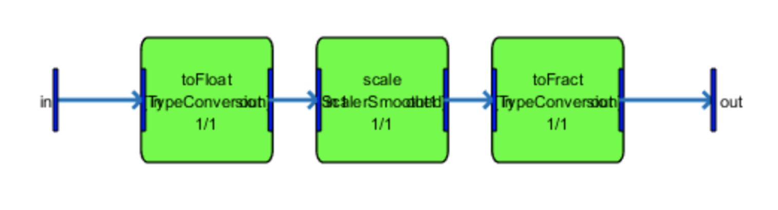
The input and output of the subsystem are represented by the narrow filled rectangles at the left and right edges of the figure. The modules are drawn as green rectangles and connections are represented by the lines with arrows. The draw command is useful for checking to make sure that the wiring of a subsystem is correct, especially complicated subsystems containing multiple modules.
Building and Running the System
The subsystem is now fully defined and ready to be run on the target. In this tutorial, we will run the subsystem natively on the PC. Issue the MATLAB command:
SYS=build(SYS);
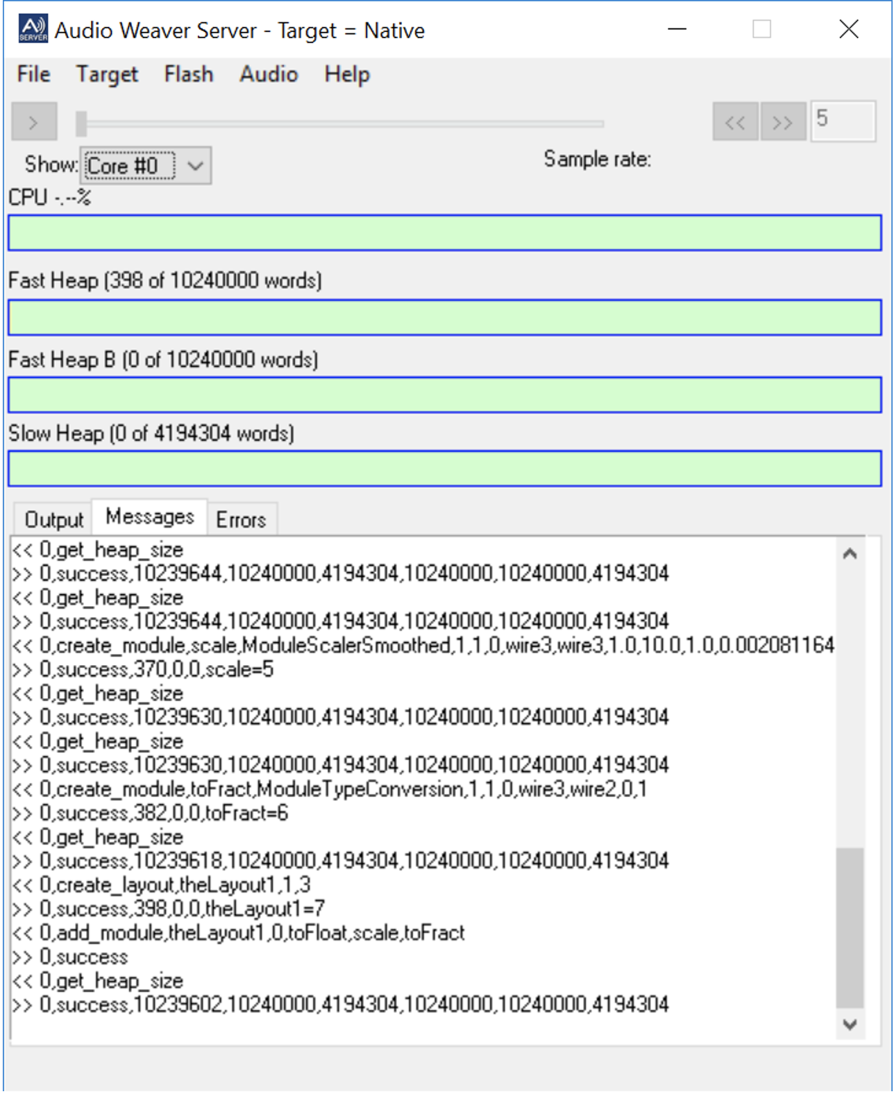
The build command begins a long sequence of events needed to instantiate the system on the target. First, it runs a routing algorithm to determine the order in which to execute the modules and then it allocates input and output buffers called “wires” to hold the data. Next the individual modules are instantiated. When done, MATLAB will report the total amount of memory required to build the system
Core 0: Total memory usage: used (left)
  Fast Heap:      398 (10239602)
 FastB Heap:        0 (10240000)
  Slow Heap:        0 ( 4194304)
Switching to the Server window messages tab, you will see that a number of commands have been sent from MATLAB to the Server:
At this point, the system has been created in the Server. The only thing left to do is enable real-time audio flow. This can be done in two different ways. First, to use the line input to the sound card, use:
awe_server_command('audio_pump');
You'll need to attach an external source, such as a CD player or MP3 player, to the line or microphone input of your PC. Alternatively, to play audio from a stored audio file, use
awe_server_command('audio_pump,../../Audio/Bach Piano.mp3');
Files can be specified with an absolute path, or a relative path, as shown above. Relative paths are addressed relative to the location of the AWE_Server executable. The command awe_server_command.m used above sends messages directly from MATLAB to the Server. The string passed is the actual message sent to the Server and you will see the string appear in the Server window.
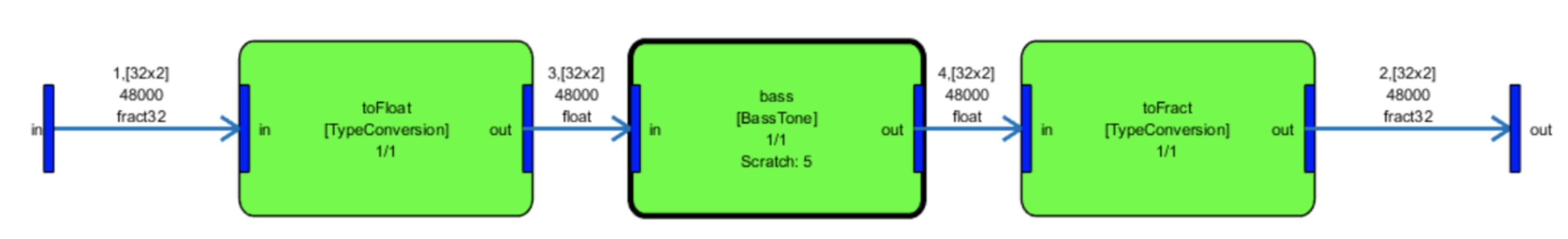
You can see the data types on the figure drawing by clicking on the toolbar button on the figure window.

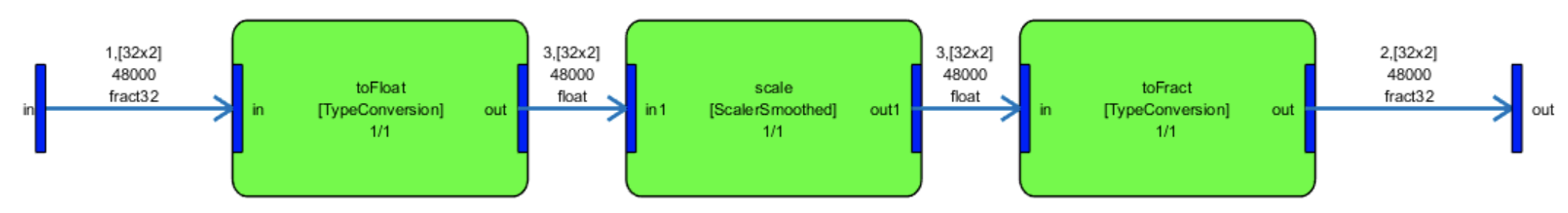
Each wire in the system is annotated with additional information. The form of the annotation is
wireIndex, [blockSize x numChannels]
              sampleRate
              dataType
where wireIndex is a unique integer identifying the wire. Wire indexes start at 1. blockSize and numChannels indicate the number of samples per block and the number of interleaved channels. In this case, we see that each wire contains two channels (stereo) with 32 samples per block. The sample rate is 48000 Hz. The data arrives as fract32, is converted to floating-point, processed by a floating-point scaler, and then converted back to fract32.
The process of determining the sizes of the pins and wires in the system is referred to as pin propogation. Essentially, the dimensions and sample rates of the input and output pins of the overall system are fixed by the target hardware. The pin information then flows from the input pins through the wires to the output of the system. At this point, we verify that the propagated output pin information matches the actual sizes of the output pins.
Real-time Tuning
At this point, the system is running in real-time on your PC. The audio source is either a file or the line input on your sound card, depending upon the audio_pump command. The scaler is configured with a gain of 0.5 and a smoothing time of 20 milliseconds.
Audio Weaver permits real-time manipulation of the system. As before, you can type MATLAB commands to manipulate the system. However, changes are now sent to the target as well. For example, to increase the gain type
SYS.scale.gain=1;
To slow down the rate of gain changes, increase the smoothing time:
SYS.scale.smoothingTime=1000;
Now ramp the gain down to zero:
SYS.scale.gain=0;
You will now hear the audio slowly fade out. You will also note that each command issued in MATLAB causes one or more messages to be sent to the Server. Similarly, if you query a value as in
X=SYS.scale.gain;
the value is read from the Server.
Audio Weaver also provides Server side user interfaces. To see the interface for the scaler, type
inspect(SYS.scale);
The following figure appears:
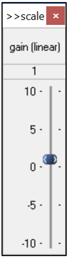
This interface is referred to as an inspector in Audio Weaver. They allow you to adjust parameters on the Server while audio is running in real-time. There are sliders for the tunable parameters: .gain and .smoothingTime. The Server is able to draw inspectors when creating systems using the MATLAB automation API and these inspectors are shown in this document. The inspectors drawn by the Designer GUI are slightly different but their functionality is equivalent.
Double-clicking on the title bar of the inspector reveals extended controls. (This feature is only available in Server drawn inspectors; not in the Designer GUI inspectors.) These controls are used infrequently and are hidden during normal use.
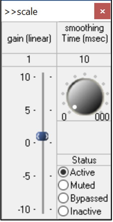
Note the control labeled "Status" found on the extended control panel. Each module has an associated run-time status with 4 possible values
Active – The module's processing function is being called. This is the default behavior when a module is first instantiated.
Muted – The module's processing function is not called. Instead, all of the output wires attached to the module are filled with zeros.
Bypassed – The module's processing function is not called. Instead, the module's input wires are copied directly to its output wires. An intelligent algorithm attempts to match up input and output wires of the same size.
Inactive – The module's processing function is not called and the output wire is untouched. This mode is used almost exclusively for debugging and the output wire is left in an indeterminate state. In this example, setting the module to Inactive will cause the contents of the output wire to be recycled resulting in a periodic 1.5 kHz whine.
Changing the module status is useful for debugging and making simple changes to the processing at run-time.
MIPS and Memory Profiling
Several other useful features are available after a system is built. You can determine the MIPs and memory load of the algorithm by the command:
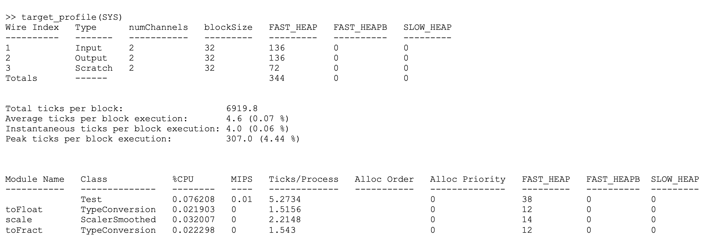
The profile indicates that the wire buffers require a total of 344 32-bit words and that the scaler module itself requires 14 32-bit words. The real-time processing load is about 0.07% of the CPU. The profile isn't that interesting for a such a small system but becomes important for complex systems.
Automatic Gain Control
In this example an automatic gain control (AGC) normalizes the output playback level independent of the level of the input audio. In addition to the AGC, the system has a volume control and input and output meters.
Begin by creating a subsystem that will execute on the target processor:
SYS=target_system('AGC Example');
Then we query the target to determine its capabilities:
T=target_get_info;
T is a data structure containing:
                    name: 'Native'
                 version: '1.0.0.5'
           processorType: 'Native'
          commBufferSize: 4105
             maxNumCores: 8
              numThreads: 4
            numInputPins: 64
           numOutputPins: 64
         isFloatingPoint: 1
        isFlashSupported: 1
                   numIn: 2
                  numOut: 2
            inputPinType: [1×1 struct]
           outputPinType: [1×1 struct]
    fundamentalBlockSize: 32
              sampleRate: 44100
               sizeofInt: 4
            profileClock: 10000000
               proxyName: 'Local'
               coreClock: 2.9040e+09
                  coreID: 0
                   isSMP: 1
             featureBits: 0
                inputPin: [0×1 containers.Map]
               outputPin: [0×1 containers.Map]
where numIn and numOut may vary depending on which sound card is in use. Using T, we then add input and output pins to the system which match the sample rate of the sound card. Both pins are stereo and have a 64 sample block size.
add_pin(SYS,'input', 'in', '' ,new_pin_type(2, 64, T.sampleRate, 'fract32'));
add_pin(SYS,'output', 'out', '', new_pin_type(2, 64, T.sampleRate, 'fract32'));
Then we add 6 modules and connect them together.
add_module(SYS, type_conversion_module('toFloat', 0));
add_module(SYS, scaler_db_module('scale'));
add_module(SYS, meter_module('inputMeter'));
add_module(SYS, agc_subsystem('agc'));
add_module(SYS, meter_module('outputMeter'));
add_module(SYS, type_conversion_module('toFract', 1));

connect(SYS, '', 'toFloat');
connect(SYS, 'toFloat', 'scale');
connect(SYS, 'scale', 'inputMeter');
connect(SYS, 'scale', 'agc');
connect(SYS, 'agc', 'toFract');
connect(SYS, 'toFract', '');
connect(SYS, 'agc', 'outputMeter');
Finally, we selectively expose some of the internal controls to create an overall inspector
SYS.scale.gainDB.range=[-20 20];
SYS.scale.gainDB.guiInfo.size=[1 3];
SYS.inputMeter.value.guiInfo.size=[1 3];
SYS.inputMeter.value.guiInfo.range=[-30 0];
SYS.outputMeter.value.guiInfo.size=[1 3];
SYS.outputMeter.value.guiInfo.range=[-30 0];

add_control(SYS, '.scale');
add_control(SYS, '.inputMeter');
add_control(SYS, '.agc.core');
add_control(SYS, '.outputMeter');
The .range field of the variable sets the range of the control slider or knob. The .size field controls its graphical size on the inspector.
Finally, build the system, draw the inspector, and start real-time audio processing.
build(SYS);
awe_inspect('position', [0 0])
inspect(SYS);
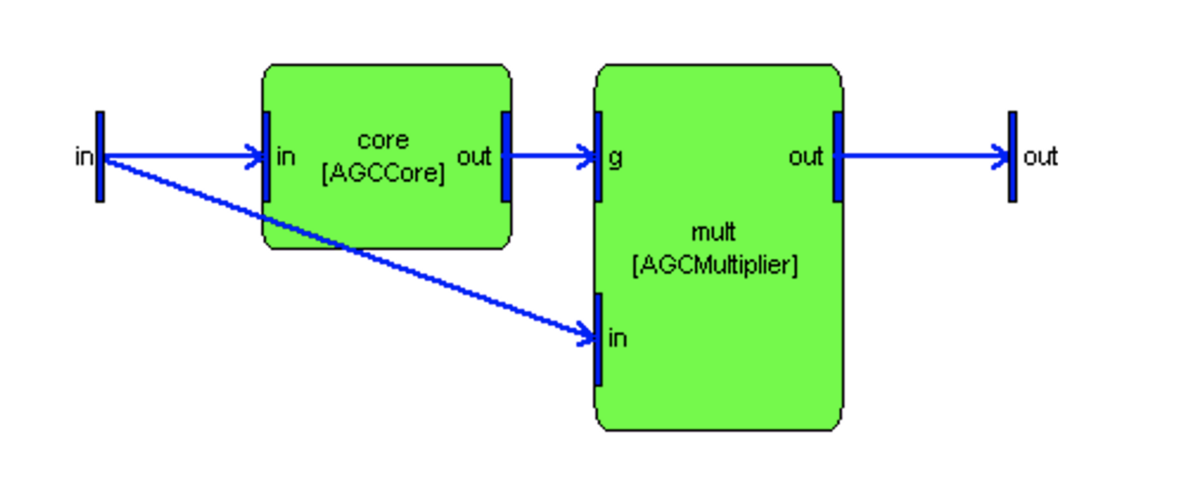
test_start_audio;The script test_start_audio.m begins real-time audio playback. On the PC, an MP3 file is used as the audio source, and on an embedded processor, the line input is the source. The final system built is shown below:
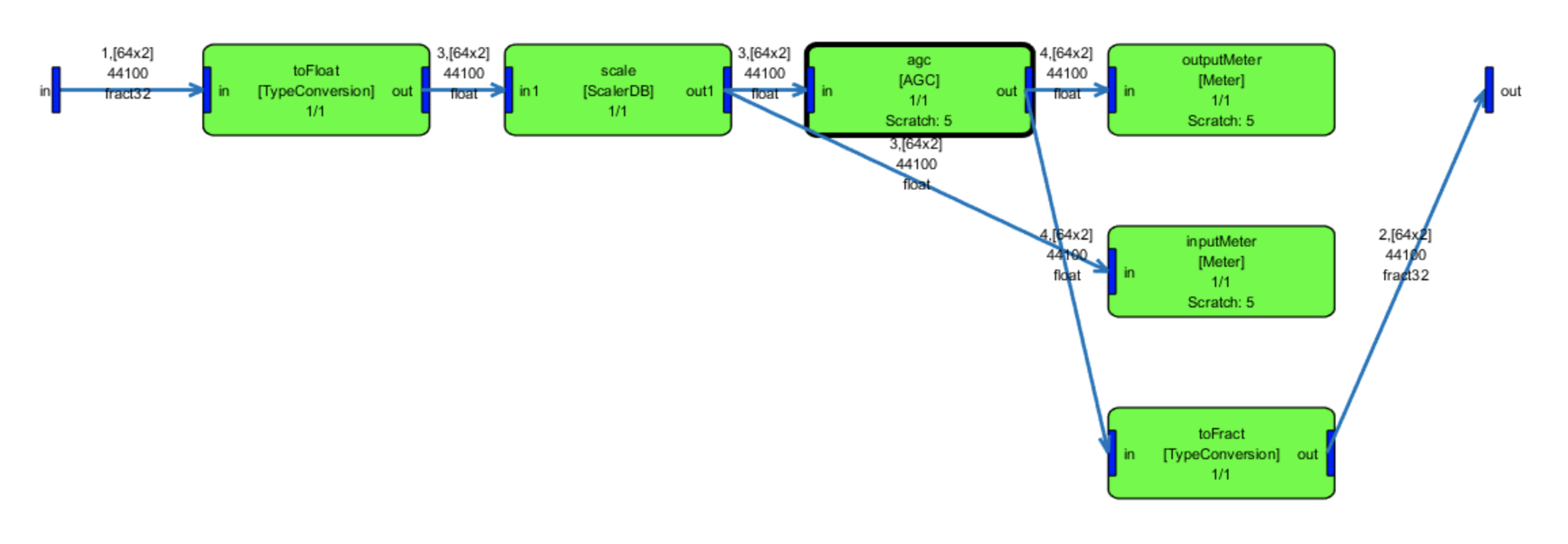
The AGC module is drawn in bold and is itself a subsystem. Peering inside, we see:
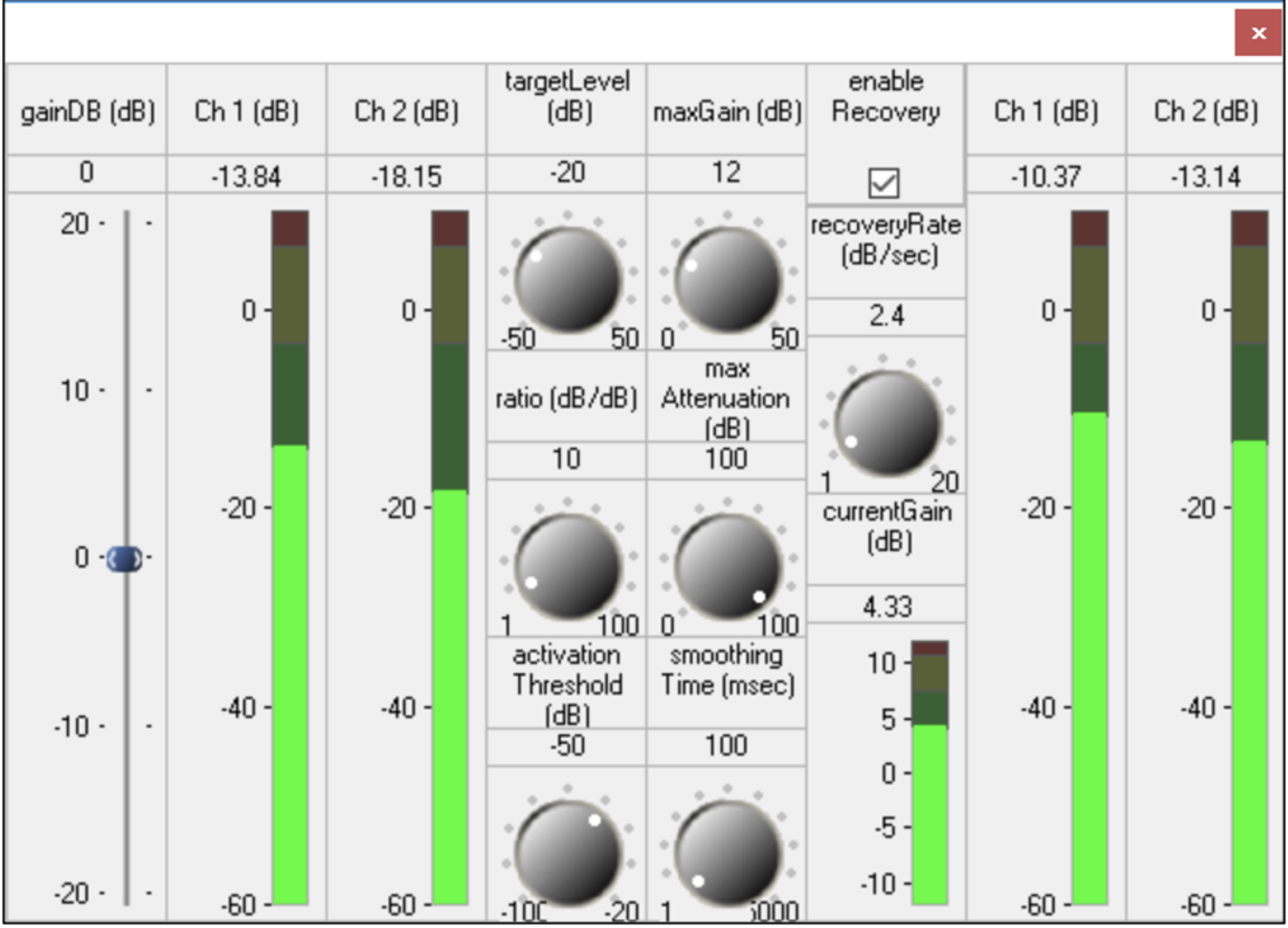
The inspector panel created is.
Bass and Treble Tone Controls
This example demonstrates how to use the second_order_filter_module.m to create bass and treble tone controls. The steps should start looking familiar. We create the overall system and then add input and output pins that match the target in terms of sample rate:
SYS=target_system('SOF Example');
T=target_get_info;
add_pin(SYS,'input', 'in', '' ,new_pin_type(2, 64, T.sampleRate, 'fract32'));
add_pin(SYS,'output', 'out', '', new_pin_type(2, 64, T.sampleRate, 'fract32'));
We then add two instances of the second_order_filter_module.m in addition to the type conversion modules. This filter is a general purpose second order filter ("Biquad") with a large number of built-in design equations. The filters are named "bass" and "treble".
add_module(SYS, type_conversion_module('toFloat', 0));
add_module(SYS, second_order_filter_module('bass'));
add_module(SYS, second_order_filter_module('treble'));
add_module(SYS, type_conversion_module('toFract', 1));
Configure the bass filter to be a low shelf. This filter is exactly what is needed for a bass tone control. Set the corner frequency of the shelf to 500 Hz. and the default gain to 0 dB.
SYS.bass.filterType=8;
SYS.bass.freq=500;
SYS.bass.gain=0;
Repeat for the treble filter but configure it as a high shelf with a corner frequency of 3 kHz.
SYS.treble.filterType=10;
SYS.treble.freq=3000;
SYS.treble.gain=0;
To connect all of the modules together.we use a special form of the connect.m command which allows us to make multiple connections with a single command. Start at the input of the system, go through the bass and treble modules, and then to the system output.
connect(SYS, '', 'toFloat', 'bass', 'treble', 'toFract', '');
Add user interface information. We'll label the sliders "bass" and "treble" and set their ranges. Then add these controls to the master inspector panel.
SYS.bass.gain.guiInfo.label='bass';
SYS.bass.gain.range=[-12 12];
SYS.treble.gain.guiInfo.label='treble';
SYS.treble.gain.range=[-12 12];
add_control(SYS, 'bass.gain');
add_control(SYS, 'treble.gain');
Finally build the system, draw the inspector, and start real-time audio playback. The awe_inspect('position', [0 0]) command specifies the screen coordinates where the inspector should be drawn. If not provided, the inspector is drawn to the right of the last inspector.
build(SYS);
awe_inspect('position', [0 0])
inspect(SYS);
test_start_audio;
Bass Tone Control Module
We now present a more complicated example. A bass tone control is created as a subsystem together with MATLAB design equations. The design equations translate high-level parameters (frequency and gain) into lower level parameters which tune the subsystem. The code in this section is contained in the file bass_tone_control_float_subsystem.m.
Notes:
A related but more complicated example, bass_tone_control_module.m, is also provided with Audio Weaver. This other version supports both floating-point and fract32 signals.
The bass tone control presented here is only to illustrate certain Audio Weaver concepts. If you need a bass tone control in your system, see the example in Bass and Treble Tone Controls.
The design equations are written in MATLAB and allow you to control the module using MATLAB scripts. However, since the control code does not exist on the target, you will be unable to draw an inspector. To take it one step further and write the control code in C requires writing a custom audio module. This is beyond the scope of this User's Guide but points you towards the benefits of writing custom audio modules.
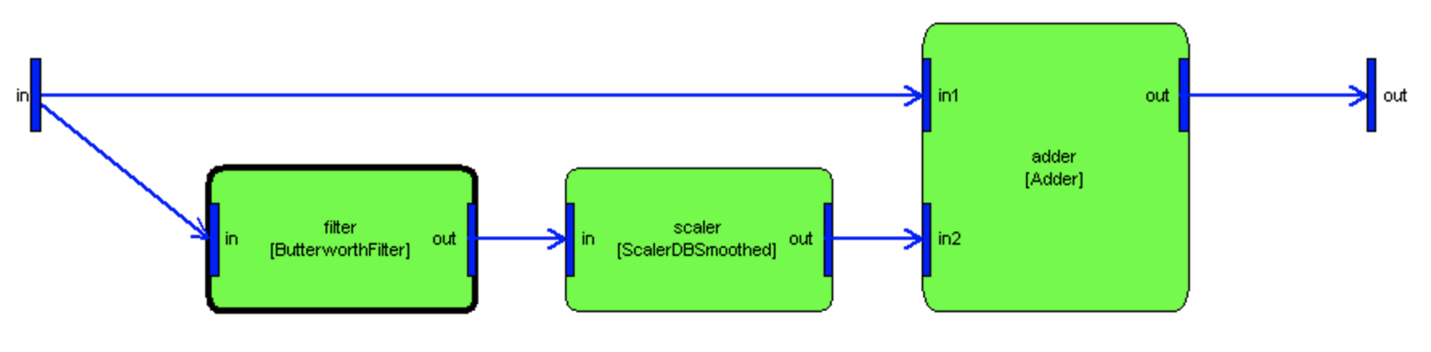
A diagram showing the overall tone control design is shown below. The design is quite simple. A first order lowpass filter is applied, scaled, and then added back to the input. When the scale equals 0 (in linear units), then the input signal is unchanged. Positive scale factors increase the amount of bass energy. Negative scale factors – up to a maximum of -1 – decrease the amount of bass energy.
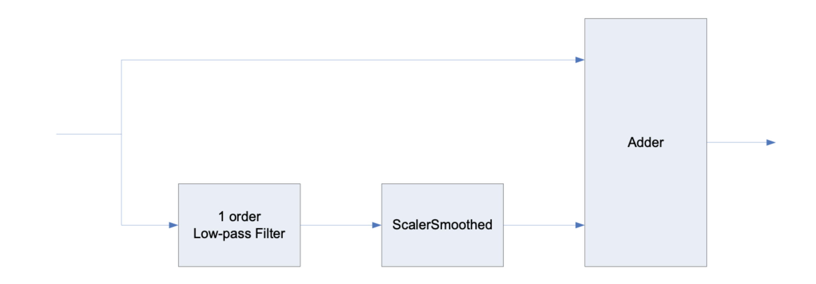
Figure 1. Schematic diagram of the bass tone control system that will be constructed as a subsystem.
The MATLAB function bass_tone_control_module.m accepts a single input argument, NAME, which is a string specifying the name of the module.
function SYS=bass_tone_control_float_subsystem(NAME)
The first step is to create a new subsystem of class “BassTone”, provide a short description, and then set the .name field of the subsystem:
SYS=awe_subsystem('BassTone', 'Bass tone control');
SYS.name=NAME;
Then we add three modules to the subsystem
add_module(SYS, butter_filter_module('filter', 1));
add_module(SYS, scaler_smoothed_module('scaler'));
add_module(SYS, adder_module('adder', 2, 0));
The first module is a first order Butterworth filter. The second module is a smoothly varying scaler that determines the amount of bass energy that is summed back in. The final module is a 2 input adder.
Next, we add input and output pins to the system. Note that no restrictions are placed on the block size, number of channels, or sample rate.
PT=new_pin_type;
add_pin(SYS, 'input', 'in', 'Audio input', PT);
add_pin(SYS, 'output', 'out', 'Audio output', PT);
and then connect the modules together:
connect(SYS, '', 'filter');
connect(SYS, 'filter', 'scaler');
connect(SYS, '.in', 'adder.in1');
connect(SYS, 'scaler', 'adder.in2');
connect(SYS, 'adder.out', '.out');
At this point, we can draw the system
draw(SYS)
and obtain the rudimentary diagram shown in Figure 2.
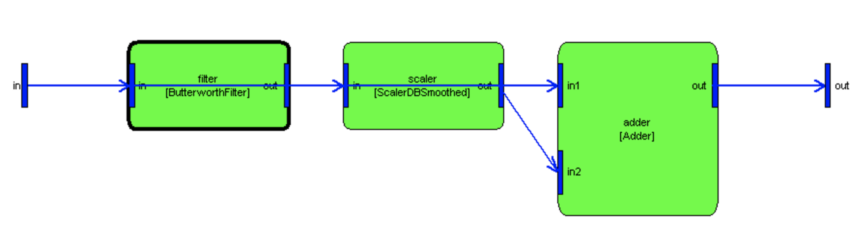
Figure 2. Bass tone control as drawn by Audio Weaver. Note that the input pin on the left has two connections: the first is to the filter and the second is to the top of the adder.
Audio Weaver isn't too smart about drawing figures. As can be seen there is some confusion because the wires overlap each other. We can nudge the adder module slightly higher in the figure with the statement:
SYS.adder.drawInfo.nudge=[0 1];
Now drawing the system, we get the more intelligible version
We are almost done. The tone control still needs an adjustable gain setting. We will define a high-level interface variable “gain” as shown below:
add_variable(SYS,'gainDB','float',0, 'parameter', 'Amount of cut/boost');
SYS.gainDB.range=[-12 12];
SYS.gainDB.units='dB';
The function add_variable(), as used here, adds a scaler to an audio module or a system. We touch upon the add_variable function here and it is fully described within the Audio Weaver Module Developers Guide. It has a number of input arguments:
SYS – the system or module to which the variable is being added.
‘gainDB’ – the name of the variable.
‘float’ – the data type of the variable. This translates directly to the variable’s C data type.
0 – the default setting of the variable.
‘parameter’ – describes the usage of the variable. Parameters are settable at run-time. ‘const’ is set at construction time and cannot change thereafter; ‘state’ is set by the processing function; 'derived' is a parameter variable that is computed based on another 'parameter'.
‘Amount of …’ – a description of what the variable does.
The next two lines set the range of the variable [-12 to +12] and the units to ‘dB’. The range is used to ensure that the variable is only set within an allowable range; the units are used for documenting the module.
The MATLAB constructor for the bass tone control is almost done. We still have:
SYS.setFunc=@bass_tone_update;
SYS=update(SYS);
 return;
The ‘@’ syntax in MATLAB is used to specify a pointer to a function. The .setFunc field of the structure specifies a MATLAB function that is called whenever a variable in the bass tone control is set. In this case, we’ll use the .setFunc to adjust the gain of the scaler based on the .gainDB field in the structure. The statement
SYS=update(SYS);
forces the .setFunc to be called once after the bass tone control is created.
Later on in the file we find the definition of the .set function:
function M=bass_tone_update(M)

gain=undb20(M.gainDB)-1;
M.scaler.gain=gain;

return;
The function bass_tone_update is a sub-function found within bass_tone_control_float_subsystem.m. The function converts the high-level .gainDB setting to a linear gain used within the scaler module. For example, if a module is instantiated and the gainDB is set to 6:
M=bass_tone_control_float_subsystem('B');
M.gainDB=6;
then scaler.gain is set to nearly 1.0:
>> M.scaler
scaler = ScalerSmoothed // Linear multichannel smoothly varying scaler

           gain: 0.995262  [linear] // Target gain
  smoothingTime: 10     [msec] // Time constant of the smoothing process
If we then set the gain to 0 dB:
>> M.gainDB=0;
we find that:
>> M.scaler
scaler = ScalerSmoothed // Linear multichannel smoothly varying scaler

           gain: 0     [linear] // Target gain
  smoothingTime: 10    [msec] // Time constant of the smoothing process
This calculation is performed by the .setFunc.
Next, we’ll run the bass tone control in real-time on the Server. Issue the following MATLAB commands:
SYS=target_system('Test', 'System containing a bass tone control');

add_pin(SYS, 'input', 'in', 'audio input', new_pin_type(2, 32, 48000, 'fract32'));
add_pin(SYS, 'output', 'out', 'audio output', new_pin_type(2, 32, 48000, 'fract32'));

add_module(SYS, type_conversion_module('toFloat', 0));
add_module(SYS, bass_tone_control_float_subsystem('bass'));
add_module(SYS, type_conversion_module('toFract', 1));

connect(SYS, '', 'toFloat', 'bass');
connect(SYS, 'bass', 'toFract', '');

SYS.bass.gainDB=6;
SYS=build(SYS);
draw(SYS);
test_start_audio;
The 5th line is of interest. It instantiates the bass tone control, names it “bass” and adds it to the system. The last line starts real-time audio processing. Once audio is flowing, you can adjust the gain of the tone control from the MATLAB prompt by setting:
SYS.bass.gainDB=12;
Note that “SYS” represents the overall system, “bass” is the bass tone control module, and “gainDB” is the high-level interface variable.
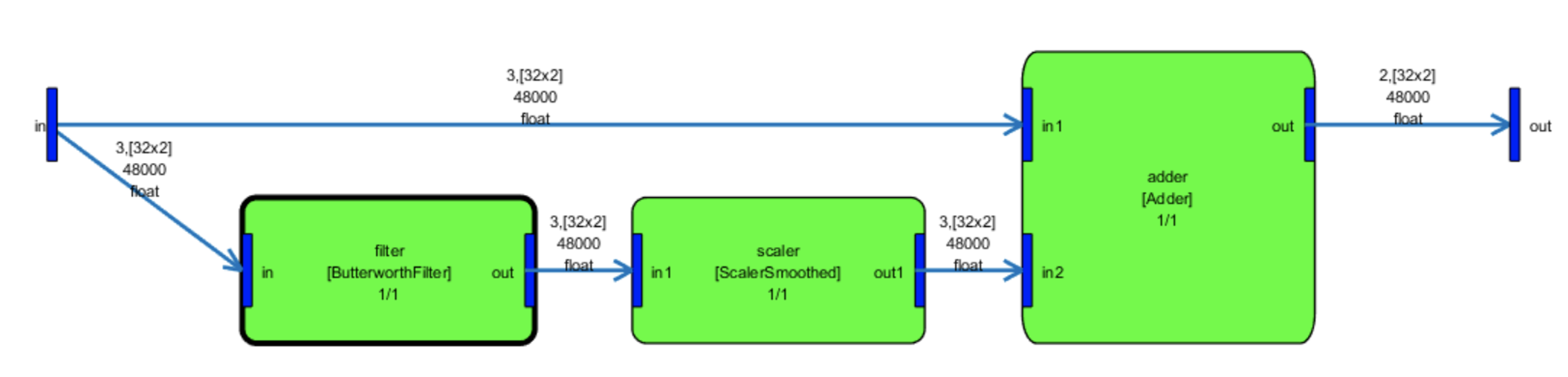
If we draw the overall system, we see a little more information displayed. First, at the high-level:
Modules with dark borders, like the bass module, indicate a subsystem. You can look inside the subsystem by right-clicking and selecting "Navigate In" or "Open in New Window", or by using the MATLAB command:
draw(SYS.bass);
Examining the bass tone control within MATLAB reveals:
>> SYS.bass
bass = BassTone // Bass tone control

  gainDB: 6         [dB] // Target gain in DB
  filter: [ButterworthFilter]
  scaler: [ScalerSmoothed]
   adder: [Adder]
The high-level variables to a subsystem are always shown first. They are followed by the internal modules. If the system is built, then the modules are reordered according to their execution order. The execution order may be different than the order that they were added to the subsystem. The process of determining execution order is referred to as routing. Routing a system also allocates all of the wires, including scratch wires. During routing, Audio Weaver reuses scratch wires in order to reduce the overall memory footprint of the algorithm.
As before, we can change the parameters of the system in real-time.
SYS.bass.gainDB=6;
changes the low frequency gain to 6 dB. We can also obtain detailed profiling information:
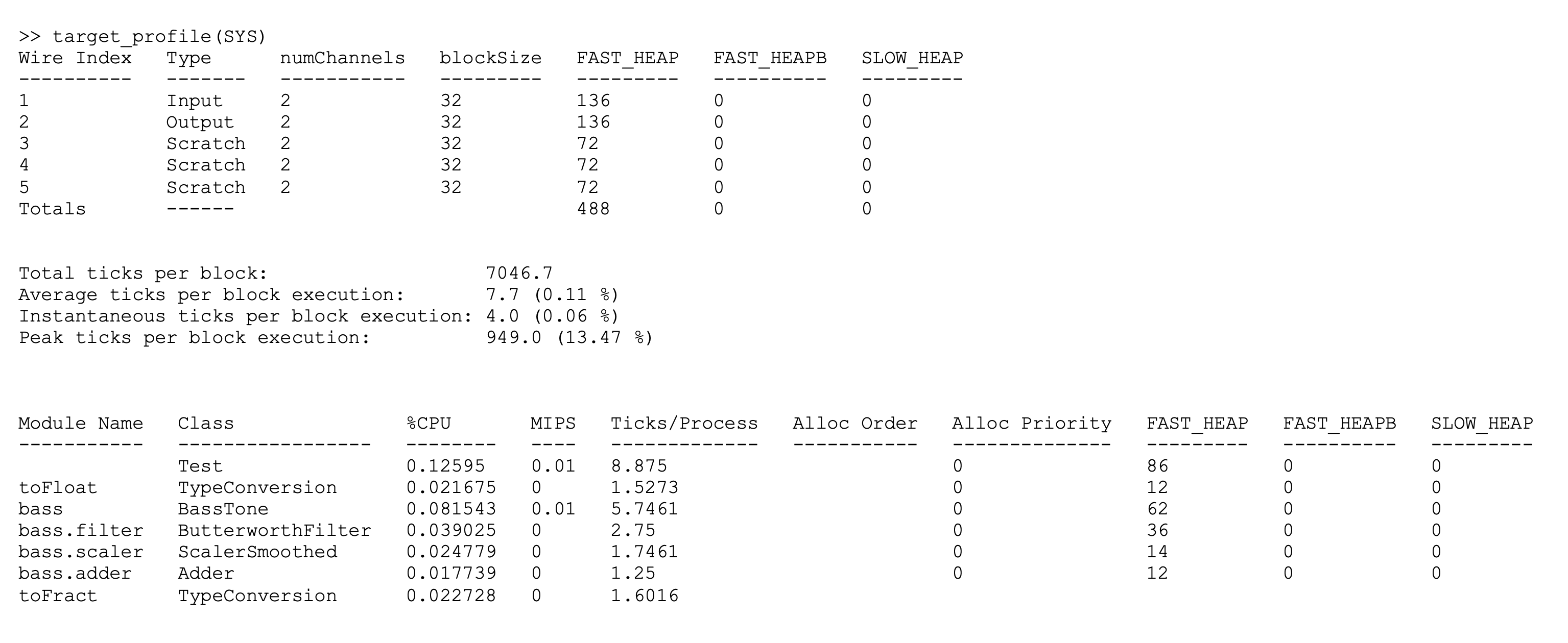
An important concept in Audio Weaver is hierarchy. Hierarchy allows you to construct more complicated audio functions out of existing pieces. The bass tone control was constructed out of lower-level modules: Butterworth filter, scaler, and an adder. In the case of the bass tone control, the hierarchy only exists within the MATLAB representation. That is, the “BassTone” class only exists in MATLAB and there is no corresponding class on the target processor. When the system is built, Audio Weaver flattens out the BassTone class into 3 separate modules. Flattening is useful because it allows us to maintain hierarchy in MATLAB without having to introduce new classes on the target processor.
Note: This guide describes high-level usage of the Audio Weaver. The code generator of Audio Weaver is able to take the bass tone control and generate code for a “BassTone” class that resides on the target. This process is described in the Custom Modules Developer's Guide.
Audio Weaver flattens the system behind the scenes while presenting the hierarchical version to the user to manipulate. To see the actual flattened system running on the target, use
draw(flatten(SYS))
You'll see that the bass tone control subsystem is gone and that its 3 internal modules have been promoted to the top level.
Key System Concepts
This section goes into further detail regarding key concepts in Audio Weaver. These were touched upon in the tutorial in Interacting with Audio Weaver Designer and The Basics of the MATLAB API, and are given full coverage here. The concepts explain how Audio Weaver operates behind the scenes and clarifies the relationship between pins, wires, modules, and subsystems.
Audio Weaver makes heavy use of MATLAB’s object oriented features. An object in MATLAB is a data structure with associated functions or methods. Each type of object is referred to as a class, and Audio Weaver uses a class to represent modules and subsystems. The class functions are stored in the directory
<AWE>\matlab\@awe_module\
It is important to understand how to use and manipulate the @awe_module class in order to properly use all of the features of Audio Weaver. Variables are also represented in Audio Weaver as objects and in early versions of Audio Weaver we used a separate awe_variable class. Recently, variables were converted to standard MATLAB structures for speed of execution. Although no longer strictly classes in MATLAB they have associated functions and methods.
@awe_module
This class represents a single primitive audio processing module or a hierarchical system. A module consists of the following components: a set of names, input and output pins, variables, and functions. All of these items exist in MATLAB and many of them have duals on the target itself.
Class Object
To create an audio module object, call the function
M=awe_module(CLASSNAME, DESCRIPTION)
The first argument, CLASSNAME, is a string specifying the class of the module. Each module must have a unique class name and modules on the Server are instantiated by referencing their class name.
Note: The function classid_lookup.m can be used to determine if a class name is already in use. Refer to Custom Modules Developer's Guide for more information.
The second argument, DESCRIPTION, is a short description of the function of the module. The DESCRIPTION string is used when displaying the module or requesting help.
After the module class is created, set the particular name of the module:
M.name='moduleName';
Note that there is a distinction between the CLASSNAME and .name of a module. The CLASSNAME is the unique identifier for the type of the module. For example, there are different class names for scalers and biquad filters. The .name identifies the module in the system. The .name field must be unique within the current level of hierarchy in the system. At this point, we have a bare module without inputs, outputs, variables, or associated functions. These must each be added.
We'll now look more closely at the fields within the @awe_module object. Instead of looking at a bare module as returned by awe_module.m, we'll look at a module that is part of a system that has already been built. We'll choose the core module within the agc subsystem:
agc_example_float;
struct(SYS.agc.core)
MATLAB displays
                      name: 'core'
                 className: 'AGCCore'
               description: 'Slowly varying RMS based gain computer'
                   classID: []
       constructorArgument: {}
               defaultName: 'AGCCore'
             moduleVersion: 30797
              classVersion: 32465
              isDeprecated: 0
             isInterpreted: 0
        nativePCProcessing: 1
                 mfilePath: 'C:\GIT\AudioWeaver\Modules\Standard\matlab\ag…'
            mfileDirectory: 'C:\GIT\AudioWeaver\Modules\Standard\matlab'
                 mfileName: 'agc_core_module.m'
                      mode: 'active'
              clockDivider: 1
                  inputPin: {[1×1 struct]}
                 outputPin: {[1×1 struct]}
                scratchPin: {}
                  variable: {1×17 cell}
              variableName: {1×17 cell}
                   control: {1×10 cell}
            wireAllocation: 'distinct'
                   getFunc: []
                   setFunc: @agc_core_set
             enableSetFunc: 0
               processFunc: @agc_core_process
                bypassFunc: @agc_core_bypass
                  muteFunc: @generic_mute
              preBuildFunc: @agc_core_prebuild_func
             postBuildFunc: []
           testHarnessFunc: @test_agc_core
               profileFunc: @profile_simple_module
               pinInfoFunc: []
                  isHidden: 0
                  isPreset: 1
                    isMeta: 0
              metaFuncName: []
           requiredClasses: {}
          consArgPatchFunc: []
             moduleBrowser: [1×1 struct]
             textLabelFunc: []
                  textInfo: [1×1 struct]
                 shapeInfo: [1×1 struct]
              freqRespFunc: []
        bypassFreqRespFunc: []
         prepareToSaveFunc: []
               copyVarFunc: @generic_copy_variable_values
               inspectFunc: []
             inspectHandle: []
           inspectPosition: []
           inspectUserData: [1×1 struct]
      numericInspectHandle: []
    numericInspectPosition: []
            freqRespHandle: []
          freqRespPosition: []
                 isTunable: 1
                      view: [1×1 struct]
                    isLive: 1
             hierarchyName: 'agc.core'
                  hasFired: 1
                targetInfo: [1×1 struct]
                    coreID: 0
        allocationPriority: 0
            isTuningSymbol: 0
                  objectID: []
           procSIMDSupport: {}
                codeMarker: {1×5 cell}
                isTopLevel: 0
       executionDependency: {}
                   presets: [1×1 struct]
               presetTable: [1×1 struct]
                numPresets: 0
                   guiInfo: [1×1 struct]
                  drawInfo: [1×1 struct]
                   uccInfo: [1×1 struct]
                   docInfo: [1×1 struct]
                  isLocked: 1
                     class: 'awe_module'
               isNavigable: 1
                    module: {}
                moduleName: {}
                connection: {}
            flattenOnBuild: 1
                 isVirtual: 0
        targetSpecificInfo: [1×1 struct]
                isPrebuilt: 1
            preProcessFunc: []
           postProcessFunc: []
                 buildFunc: []
                fieldNames: {89×1 cell}
The complete list of fields is described in the Audio Weaver Module Developers Guide. Some commonly used fields are described below.
inputPin – cell array of input pin information. This information is set by the add_pin.m function and should not be changed. You can access this field to determine the properties of the input pins. Each cell value contains a data structure such as
>> SYS.agc.core.inputPin{1}
                   type: [1×1 struct]
                  usage: 'input'
                   name: 'in'
            description: 'Audio input'
         referenceCount: 0
             isFeedback: 0
            isReuseable: 1
    initialFeedbackData: []
               pinArray: 0
               baseName: 'in'
                isDummy: 0
             showLegend: 0
           clockDivider: 1
               drawInfo: [1×1 struct]
                uccInfo: [1×1 struct]
                guiInfo: [1×1 struct]
              wireIndex: 1
              buildInfo: [1×1 struct]
          srcConnection: {}
          dstConnection: {[1×1 struct]}
           classVersion: 32555
             targetInfo: [1×1 struct]
outputPin – similar to inputPin. It is a cell array describing the output pins.
scratchPin - similar to inputPin. It is a cell array describing the scratch pins.
isHidden – Boolean specifying whether the module should be shown when part of a subsystem. Similar to the .isHidden field of awe_variable objects. User editable.
isPreset – Boolean that indicates whether a module will be included in generated presets. By default, this is set to 1 and the module becomes part of the preset. User editable.
Input, Output, and Scratch Pins
Pins are added to a module by the add_pin.m function. Each pin has an associated Pin Type as described in Pins. After creating the Pin Type, call the function
add_pin(M, USAGE, NAME, DESCRIPTION, TYPE, numPinArray)
for each input, output, or scratch pin you want to add. The arguments are as follows:
M - @awe_module object.
USAGE – string specifying whether the pin is an ‘input’, ‘output’, or 'scratch'.
NAME – short name which is used as a label for the pin.
DESCRIPTION – description of the purpose or function of the pin.
TYPE – Pin Type structure.
numPinArray – non negative integer to specify the number of pins to add. If numPinArray > 0, then this pin is considered a pin array. Pin arrays will have the naming convention of NAME<n> where n will start at 1 and stop at numPinArray. If numPinArray = 0 or is left empty, then the pin is assumed to be a scalar pin. The property PIN.pinArray can be checked to see if a PIN is a scalar pin or part of a pin array. A scalar pin's .pinArray property will be 0. A pin array's .pinArray property will be numPinArray, that is, the size of the pin array.
M.inputPin, M.outputPin, and M.scratchPin are cell arrays that describe the pins. Each call to add_pin.m adds an entry to one of these arrays, depending upon whether it is an input, output, or scratch pin.
Memory that needs to be persisted by a module between calls to the processing function appears in the instance structure and has usage "state". However, some processing functions require temporary memory storage. This memory is only needed while processing is active and does not need to be persisted between calls. The mechanism for allocating this temporary memory and sharing it between modules is accomplished by scratch pins. Scratch pins are added to a module via add_pin.m with the USAGE argument set to 'scratch'. Scratch pins are not typically used by audio modules, but are often required by subsystems. For subsystems, the routing algorithm automatically determines scratch pins at build time.
Variables
Every audio module has an associated set of variables. These variables are shown in MATLAB and also appear on the target as well. All of a module’s variables exist in both MATLAB and on the target processor.
Use the add_variable.m command to add variables to an audio module. The short syntax is:
add_variable(M, VAR)
where M is the @awe_module object and VAR is the awe_variable object. Using the short syntax requires that the variable object already be constructed. The longer and more useful syntax for adding a variable is:
add_variable(M, NAME, TYPE, VALUE, USAGE, DESCRIPTION, ISHIDDEN, ISCOMPLEX);
where the 2nd and subsequent arguments are passed to the awe_variable.m function. See @awe_module for a description of these parameters.
After adding a variable to an audio module, it is a good idea to also specify its range and units. The range field is used when drawing user interfaces (sliders and knobs, in particular) and also for validating variable assignments. The units string reminds the user of what units the variable represents. You set these as:
M.variableName.range=[min max];
M.variableName.units='msec';
Note that after a variable is added to a module, it appears as a field within the module’s structure and the name of the field equals the name of the variable. Attributes of an individual variable are referenced using the “.” structure notation.
As an example, let’s look at the variables within the scaler_smoothed_example_module.m function. We see:
add_variable(M, 'gain', 'float', 0, 'parameter', 'Target gain');
M.gain.range=[-10 10];
M.gain.units='linear';

add_variable(M, 'smoothingTime', 'float', 10, 'parameter', 'Time constant of the smoothing process');
M.smoothingTime.range=[0 1000];
M.smoothingTime.units='msec';

add_variable(M, 'currentGain', 'float', M.gain, 'state', 'Instantaneous gain applied by the module.  This is also the starting gain of the module.', 1);

add_variable(M, 'smoothingCoeff', 'float', NaN, 'derived', 'Smoothing coefficient', 1);
Only the first two variables, .gain, and .smoothingTime are visible and thus need range and units information. The variable smoothingCoeff is initially set to NaN (“not a number” which is a valid floating-point value) and is set to its true value by the module’s set function.
Array variables are handled in a similar fashion except that all arrays are indirect arrays - the instance structure type definition contains a pointer to the array. For example, an FIR filter has separate arrays for coefficients and state variables:
add_variable(M, 'numTaps', 'int', L, 'const', 'Length of the filter');
M.numTaps.range=[1 5000 1];
M.numTaps.units='samples';

add_array(M, 'coeffs', 'float', [1; zeros(L-1,1)], 'parameter', 'Coefficient array');
M.coeffs.arrayHeap='AE_HEAP_FAST2SLOW';
M.coeffs.arraySizeConstructor='S->numTaps * sizeof(float)';

add_variable(M, 'stateIndex', 'int', 0, 'state', 'Index of the oldest state variable in the array of state variables');
M.stateIndex.isHidden=1;

% Set to default value here.  This is later updated by the pin function
add_array(M, 'state', 'float', zeros(L, 1), 'state', 'State variable array');
M.state.arrayHeap='AE_HEAP_FASTB2SLOW';
M.state.arraySizeConstructor='ClassWire_GetChannelCount(pWires[0]) * S->numTaps * sizeof(float)';
M.state.isHidden=1;
Subsystem Constructor Function
The call to create a new empty subsystem is similar to the call to create a new module described in @awe_module
SYS=awe_subsystem(CLASSNAME, DESCRIPTION);
You have to provide a unique class name and a short description of the function for the subsystem. (To be precise, the CLASSNAME only has to be unique if you are generating C code with the new subsystem class. Then, the CLASSNAME has to be unique among all of the subsystems and audio modules.)
After the subsystem is created, set the particular name of the subsystem:
SYS.name='subsystemName';
At this point, we have an empty subsystem; no modules, pins, variables, or connections. Pins and variables are added using add_pin.m and add_variable.m just as for @awe_module objects.
Adding Modules
Modules are added to subsystems one at a time using the function
add_module(SYS, MOD)
The first argument is the subsystem while the second argument is the module (or subsystem) to add. Once a module is added to a subsystem, it appears as a field within the object SYS. The name of the field is set to the module's name. Modules can be added to subsystems in any order. The run-time execution order is determined by the routing algorithm.
As modules are added to the subsystem, they are appended to the .module field. You can use standard MATLAB programming syntax to access this information. For example, to determine the number of modules in a subsystem:
count=length(SYS.module);
Or, to print out the names of all of the modules in a subsystem:
for i=1:length(SYS.module)
       fprintf(1, '%s\n', SYS.module{i}.name);
end
Adding Pins
The syntax for adding input and output pins to subsystems mirrors the syntax for adding these items to modules. Refer to Input, Output, and Scratch Pins for the details. Scratch pins are frequently used by subsystems to hold intermediate wire buffers between modules. Fortunately, allocating these temporary connections between modules is handled automatically by the routing algorithm. There is no need to add scratch pins to subsystems.
In some cases, you want to add a pin to a subsystem that is of the same type as an internal module. For example, the Hilbert subsystem uses the same pin type as the Biquad filter. This can be achieved programmatically as shown below:
add_module(SYS, biquad_module('bq11'));
pinType=SYS.bq11.inputPin{1}.type;

add_pin(SYS, 'input', 'in', 'Audio Input', pinType);
add_pin(SYS, 'output', 'out', 'Audio output', pinType);
Adding Variables
Variables are added to subsystems in the same manner as they are added to modules. Refer to Variables for the details.
Making Connections
Connections between modules are specified using the connect.m command. The general form is:
connect(SYS, SRCPIN, DSTPIN);
where SRCPIN and DSTPIN specify the source and destination pins, respectively. Pins are specified as strings to the connect.m command using the syntax:
moduleName.pinName
Consider the system shown below that is contained within multiplexor_example.m.
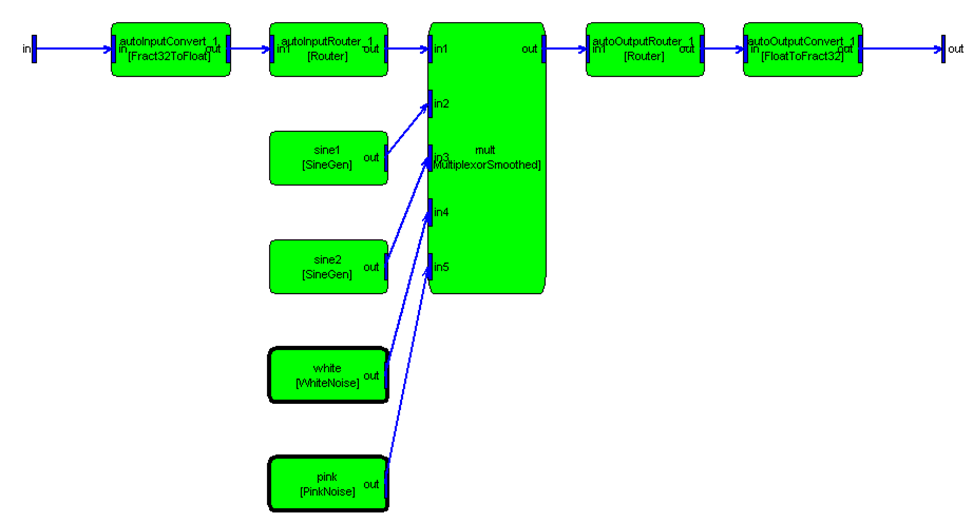
To connect the output of the sine generator1 to the second input of the multiplexor, use the command:
connect(SYS, 'sine1.out', 'mult.in2');
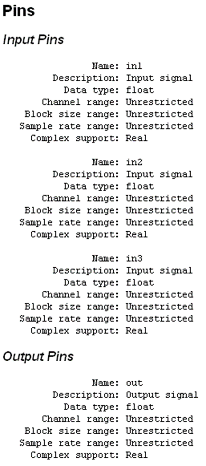
The module names "sine1" and "mult" are obvious because they were specified when the modules were created. The pins names may not be obvious since they appear within the module's constructor function. To determine the names of a module's pins, you can either utilize the detailed help function awe_help described in Online Help (recommended)
awe_help multiplexor_smoothed_module
or have MATLAB draw the module
M=multiplexor_smoothed_module('foo');
draw(M)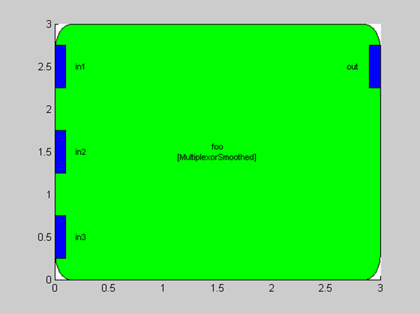
Several short cuts exist to simplify use of the connect command.
If the module has only a single input or output pin, then you need only specify the module name; the pin name is assumed. Since the sine wave generator module in the multiplexor example has only a single output pin, the example above reduces to:
connect(SYS, 'sine1', 'mult.in2');
Inputs and outputs to the subsystem are specified by the empty string. Thus,
connect(SYS, '', 'mult.in1');
connects the input of the system to the first input of the multiplexor. Similarly,
connect(SYS, 'mult', '');
connects the output of the multiplexor to the output of the system.
By default, the connect command performs rudimentary error checking. The function verifies that the named modules and pins exist within the subsystem. At build time, however, exhaustive checking of all connections is done. Audio Weaver verifies that all connections are made to compatible input and output pins (using the range information within the pin type).
Output pins are permitted to fan out to an arbitrary number of input pins. Input pins, however, can only have a single connection.
Audio Weaver is setup to handle several special cases of connections at build time. First, if an input pin is unconnected, Audio Weaver will insert a source module and connect it to the unconnected input. Either a source_module.m (float) or source_fract32_module.m is added based on the first input to the system.
Note: Audio Weaver is guessing at the type of pin that needs to be connected.
If a module has an unconnected output pin, Audio Weaver inserts a sink module based on the data type of the unconnected pin.
sink_module.m	Floating-point data
sink_fract32_module.m	Fixed-point data
sink_int_module.m	Integer data
Note: This is always correct since the pin type is inherited from the module's output pin.
If the subsystem has a direct connection from an input pin to an output pin, then a copier_module is inserted. If a module output fans out to N outputs of the subsystem, then N-1 copier modules are inserted.
Note: This is required since each output of the subsystem is stored in a separate buffer.
Top-Level Systems
Thus far, we have been using the terms system and subsystem interchangeably. There is a slight difference, though, that you need to be aware of. The highest level system object that is passed to the build command must be a top-level system created by the function:
SYS=target_system(CLASSNAME, DESCRIPTION, RT)
The top-level system is still an @awe_subsystem object but it is treated differently by the build process. The main difference is how the output pin properties are handled. In a top-level system, the output pins properties are explicitly specified and not derived from pin propagation. As an added check, the pin propagation algorithm verifies that the wires attached to a top-level system's output pins match the properties of each output pin of the target. The top-level system functions are described in more detail in target_system.m and matlab_target_system.m.
In contrast, internal subsystems are created by calls to
SYS=awe_subsystem(CLASSNAME, DESCRIPTION)
.awe_variable objects
A variable in Audio Weaver represents a single scalar or array variable on the target processor. Variables are added to modules or subsystems using the add_variable.m command described in the Audio Weaver Module Developers Guide. Even if you are not developing modules, it is good to understand the awe_variable object so that you can fully utilize variables.
A new scalar variable is created by the call:
awe_variable(NAME, TYPE, VALUE, USAGE, DESCRIPTION, ISHIDDEN, ISCOMPLEX)
Variables in Audio Weaver have a close correspondence to variables in the C language. We have:
NAME – name of the variable as a string.
TYPE – C type of the variable as a string. For example, ‘int’ or ‘float’.
VALUE – initial value of the variable.
USAGE – a string specifying how the variable is used in Audio Weaver. Possible values are:
‘const’ – the variable is initialized when the module is allocated and does not change thereafter.
‘parameter’ – the variable can be changed in real-time and is exposed as a control.
‘derived' – similar to a parameter, but the value of the variable is computed based on other parameters in the module. Derived variables are not normally exposed as controls.
‘state’ – the variable is set in real-time by the processing function.
DESCRIPTION – a string describing the function of the variable.
ISHIDDEN – an optional Boolean indicating whether the variable is visible (ISHIDDEN=0) or hidden (ISHIDDEN=1). By default, ISHIDDEN=0.
ISCOMPLEX – an optional Boolean indicating whether the variable is real valued (ISCOMPLEX=0) or complex (ISCOMPLEX=1). By default, ISCOMPLEX=0.
You typically do not use the awe_variable function directly. Rather, the function is automatically called when you add variables to modules or subsystems using the add_variable.m function.
M=add_variable(M, VAR1, VAR2, ...)
The first argument to add_variable.m is the module or subsystem, and all subsequent arguments are passed directly to the awe_variable.m function.
The add_variable.m function is used to add scalar variables. Use the function
add_array(M, NAME, TYPE, VALUE, USAGE, DESCRIPTION, ISHIDDEN, ISCOMPLEX);
to add arrays. Audio Weaver supports 1 and 2 dimensional arrays. The 2-dimensional array representation is maintained in MATLAB. On the target, however, a 2-dimensional array is flattened into a 1-dimensional array on a column by column basis. Both scalar and array variables are represented as awe_variable objects.
We now look carefully at one of the variables in the agc_example.m system. At the MATLAB prompt, type:
agc_example_float;
get_variable(SYS.agc.core, 'targetLevel')
The get_variable.m command extracts a single variable from a module and returns the @awe_module object. (If you instead try to access SYS.agc.core.targetLevel you'll only get the value of the variable, not the actual structure.) You'll see:
                    name: 'targetLevel'
           hierarchyName: 'agc.core.targetLevel'
                   value: -20
                    size: [1 1]
                    type: 'float'
               isComplex: 0
                   range: [-50 50 0.1000]
              isVolatile: 0
                   usage: 'parameter'
             description: 'Target audio level.'
               arrayHeap: 'AWE_HEAP_FAST2SLOW'
           memorySegment: 'AWE_MOD_FAST_ANY_DATA'
    arraySizeConstructor: ''
         constructorCode: ''
                 guiInfo: [1x1 struct]
                  format: '%g'
                   units: 'dB'
                  isLive: 1
                isHidden: 0
                 presets: [1x1 struct]
                 isArray: 0
              targetInfo: [1x1 struct]
                isLocked: 1
                   isPtr: 0
                 ptrExpr: ''
         isRangeEditable: 1
          isTuningSymbol: 0
             isTextLabel: 1
                isPreset: 1
             isDisplayed: 1
            classVersion: 29341
                   class: 'awe_variable'
              fieldNames: {32x1 cell}
We describe some of the fields which are commonly edited here. Refer to Custom Modules Developer's Guide for a complete description.
range – a vector or matrix specifying the allowable range of the variable. This is used to validate variable updates and also to draw knobs and sliders. This vector uses the same format as the pin type described in Section 4.1.3. User editable.
For example, the SYS.agc.core.targetLevel variable has the default range
>> SYS.agc.core.targetLevel.range

ans =

   -50    50
and this is used to set the range of the inspector knob. You can change the range to +/- 10 dB by setting
SYS.agc.core.targetLevel.range=[-10 10]
prior to drawing the inspector.
format - C formatting string used by sprintf when displaying the value as part of a module. Follows the formatting conventions of the C printf function. User editable.
For example, the default format for the .targetLevel variable is '%g'. When you display the module in the MATLAB output window, you see
>> SYS.agc.core
core = AGCCore // Automatic Gain Control gain calculator module

          targetLevel: -20       [dB] // Target audio level
       maxAttenuation: 100       [dB] // Maximum attenuation of the AGC
              maxGain: 12        [dB] // Maximum gain of the AGC
                 ...
If you change the format to:
SYS.agc.core.targetLevel.format='%.2f'
then MATLAB will display
core = AGCCore // Automatic Gain Control gain calculator module

          targetLevel: -20.00    [dB] // Target audio level
       maxAttenuation: 100       [dB] // Maximum attenuation of the AGC
              maxGain: 12        [dB] // Maximum gain of the AGC
Note that the .format field does not effect how the variable is displayed when returned to MATLAB, as in
SYS.agc.core.targetLevel
In this case, Audio Weaver returns the numerical value of .targetLevel to MATLAB and let's MATLAB determine how to display it.
units - a string containing the underlying units of the variable. For example, ‘dB’ or ‘Hz’. This is used by documentation and on user interface panels. User editable.
isLive – Boolean variable indicating the variable is residing on the target (isLive = 1), or if it has not yet been built (isLive=0). This starts out with a value of 0 when the module is instantiated and is then set to 1 by build.m. Not user editable.
isHidden – Boolean indicating whether a variable is hidden. Hidden variables are not shown when a subsystem is displayed in the MATLAB output window. However, hidden variables may still be referenced. User editable.
The .isHidden field can be used to hide variables that the user typically does not interact with. For example, allocate a 2nd order Biquad filter:
>> M=biquad_module('filter')
filter = Biquad // 2nd order IIR filter

  b0: 1          // First numerator coefficient
  b1: 0          // Second numerator coefficient
  b2: 0          // Third numerator coefficient
  a1: 0          // Second denominator coefficient
  a2: 0          // Third denominator coefficient
All 5 of the tunable filter coefficients are shown. After the filter is built, state variables are added. You can see them by typing:
>> M.state

ans =

     0
     0
Of course, this assumes that you know what the variables are called. To automatically show hidden variables in the MATLAB output window, set
AWE_INFO.displayControl.showHidden=1;
Then, looking at the Biquad filter, all of the hidden variables will be automatically shown:
filter = Biquad // 2nd order IIR filter

     b0: 1          // First numerator coefficient
     b1: 0          // Second numerator coefficient
     b2: 0          // Third numerator coefficient
     a1: 0          // Second denominator coefficient
     a2: 0          // Third denominator coefficient
  state: 0
          0]
See AWE_INFO for a description of all user settable fields in the AWE_INFO structure.
Advanced Variables: add_argument()
There are certain cases where runtime tunable parameters do not contain enough information for correctly sizing memory blocks within a system. Arguments are created from information passed in at module creation. An example for using an argument is usually to set an upper bound for runtime memory such as to set a maxDelay parameter on a delay module. This can allow the user to set a max delay at construction time, and then use a runtime delay setting bounded by maxDelay. Guidelines for module arguments are as follows:
Do not use arguments that are already available on input pins like number of channels or block sizes
For the argument to be accessible it must be tracked with a const variable:
function M=user_delay_module(NAME, MAXDELAY)
…
% add an argument with the constructor input MAXDELAY
add_argument(M, 'maxDelay', 'int', MAXDELAY, 'const', 'Maximum delay, in samples');
%add a variable to track the max delay in code (the name can be the same, constructor %arguments are stored in a separate container
add_variable(M, 'maxDelay', 'int', MAXDELAY, 'const', 'Maximum delay, in samples.’);
%add a variable dependent on the MAXDELAY
add_array(M, 'state', 'float', [], 'state', 'State variable array.');
%add a current delay setting
add_variable(M, 'currentDelay', 'int', 0, 'parameter', 'Current delay.');
%bound the variable with MAXDELAY
M.currentDelay.range=[0 MAXDELAY 1];
M.currentDelay.isRangeEditable=0;
Use the const variable in prebuild for re-sizing
function M=user_delay_prebuild_func(M)
…
numChannels = M.inputPin{1}.type.numChannels;
M.state.size = [numChannels M.maxDelay+1];
…

•	Access arguments via the constructorArgument member:
add_argument(M, 'myOption', 'int', MYOPTION, 'const', 'Some optional argument');
M.constructorArgument{end}.guiInfo.controlType='checkBox';
More detailed information for add_argument() is in Custom Modules Developer's Guide.
Pins
The function new_pin_type.m was introduced in Adding I/O Pins and returns a data structure representing a pin. The internal structure of a pin can be seen by examining the pin data structure. At the MATLAB command prompt type:
new_pin_type
Be sure to leave off the trailing semicolon – this causes MATLAB to display the result of the function call. We see:
ans =

         numChannels: 1
           blockSize: 32
          sampleRate: 48000
            dataType: 'float'
           isComplex: 0
    numChannelsRange: []
      blockSizeRange: []
     sampleRateRange: []
       dataTypeRange: {'float'}
      isComplexRange: 0
             guiInfo: [1x1 struct]
    initialValueReal: []
    initialValueImag: []
        classVersion: 29350
The first 5 fields of the data structure specify the current settings of the pin; the next 5 fields represent the allowable ranges of the settings. The range information is encoded using the convention:
[] – the empty matrix indicates that there are no constraints placed on the range.
[M] – a single value indicates that the variable can only take on one value.
[M N] – a 1x2 row vector indicates that the variable has to be in the range M <=x <= N.
[M N step] – a 1x3 row vector indicates that the variable has to be in range M<=x<=N and that it also has to increment by step. In MATLAB notation, the set of allowable values is [M:step:N].
By default, the new_pin_type.m function returns a pin with no constraints on the sampleRate, blockSize, and numChannels. The dataType is constrained to be floating-point and the data must be real.
Additional flexibility is built into the range constraints. Instead of just a row vector, range can have a matrix of values. Each row is interpreted as a separate allowable range. For example, suppose that a module can only operate at the sample rates 32 kHz, 44.1 kHz, and 48 kHz. To enforce this, set the sampleRateRange to [32000; 44100; 48000]. Note the semicolons which place each sample rate constraint on a new row.
Audio Weaver also interprets NaN’s in the matrix as if they were blank. For example, suppose a module can operate at exactly 32 kHz or in the range 44.1 to 48 kHz. To encode this, set sampleRateRange=[32000 NaN; 44100 48000].
The new_pin_type.m function accepts a number of optional arguments:
new_pin_type(NUMCHANNELS, BLOCKSIZE, SAMPLERATE, DATATYPE, ISCOMPLEX);
These optional arguments allow you to properties of the pin. For example, the call
new_pin_type(2, 32, 48000)
returns the pin
ans =

         numChannels: 2
           blockSize: 32
          sampleRate: 48000
            dataType: 'float'
           isComplex: 0
    numChannelsRange: 2
      blockSizeRange: 32
     sampleRateRange: 48000
       dataTypeRange: {'float'}
      isComplexRange: 0
             guiInfo: [1x1 struct]
    initialValueReal: []
    initialValueImag: []
        classVersion: 29350
This corresponds to exactly 2 channels with 32 samples each at 48 kHz.
The pin type is represented using a standard MATLAB structure. You can always change the type information after new_pin_type.m is called. For example,
PT=new_pin_type;
PT.sampleRateRange=[32000; 44100; 48000];
The current values and ranges of values are both provided in Audio Weaver for a number of reasons. First, the range information allows an algorithm to represent and validate the information in a consistent manner. Second, the pin information is available to the module at design time, allocation time, and at run-time. For example, the sample rate can be used to compute filter coefficients given a cutoff frequency in Hz. Third, most modules in Audio Weaver are designed to operate on an arbitrary number of channels. The module's run-time function interrogates its pins to determine the number of channels and block size, and processes the appropriate number of samples.
Consider the bass tone control subsystem introduced in Bass Tone Control Module. The subsystem was connected to stereo input and output pins and thus all of the internal wires hold two channels of information. If the bass tone control were connected to a mono input, then all of the internal wires would be mono and the module would operate as expected. This generality allows you to design algorithms which operate on an arbitrary number of channels with little added complexity.
Usage of new_pin_type.m is slightly more complicated than described above. In fact, the 5 arguments passed to the function actually specify the ranges of the pin properties and the current values are taken as the first item in each range. For example, consider a module that can operate on even block sizes in the range from 32 to 64. This is specified as:
new_pin_type([], [32 64 2])

         numChannels: 1
           blockSize: 32
          sampleRate: 48000
            dataType: 'float'
           isComplex: 0
    numChannelsRange: []
      blockSizeRange: [32 64 2]
     sampleRateRange: []
       dataTypeRange: {'float'}
      isComplexRange: 0
             guiInfo: [1x1 struct]
    initialValueReal: []
    initialValueImag: []
        classVersion: 29350
Note that the first argument, the number of channels, is empty. An empty matrix places no constraints on the item. Notice also that the current blockSize equals the first value, 32, in the range of allowable block sizes. Additional examples highlight other ways to use this function.
You can also specify that a pin hold either floating-point or fract32 data. Pass in a cell array of strings as the 4th argument to new_pin_type:
>> P=new_pin_type([], [], [], {'float', 'fract32'})

P =

         numChannels: 1
           blockSize: 32
          sampleRate: 48000
            dataType: 'float'
           isComplex: 0
    numChannelsRange: []
      blockSizeRange: []
     sampleRateRange: []
       dataTypeRange: {'float'  'fract32'}
      isComplexRange: 0
             guiInfo: [1x1 struct]
    initialValueReal: []
    initialValueImag: []
        classVersion: 29350
Some modules do nothing more than move data around. Examples include the interleave_module.m and the delay_module.m. These modules do not care about the data type, only that it is 32-bits wide. The new_pin_type.m function uses the shorthand '*32' to represent all 32-bit data type. This currently includes 'float', 'fract32', and 'int':
>> PT=new_pin_type([], [], [], '*32')

PT =

         numChannels: 1
           blockSize: 32
          sampleRate: 48000
            dataType: 'float'
           isComplex: 0
    numChannelsRange: []
      blockSizeRange: []
     sampleRateRange: []
       dataTypeRange: {'float'  'int'  'fract32'}
      isComplexRange: 0
             guiInfo: [1x1 struct]
    initialValueReal: []
    initialValueImag: []
        classVersion: 29350
Automatic Assignment in the Calling Environment
The standard MATLAB programming model is to pass parameters by value. If a function updates one of its input arguments, then it must be returned as an output argument for the change to occur in the calling environment. For example, the add_module.m function takes an audio module as an argument and adds it to an existing subsystem. The syntax is:
SYS=add_module(SYS, MODULE)
where SYS is an @awe_subsystem object and MODULE is an @awe_module object. You'll note that SYS appears as both an input and output argument to the function add_module.m.
In some cases, Audio Weaver overrides the default MATLAB behavior in order to simplify the scripts. The function add_module.m can be called without an output argument
add_module(SYS, MODULE)
in which case the variable SYS is automatically updated in the calling environment. This works properly as long as SYS is not derived from an intermediate reference or calculation. For example, suppose that SYS contains an internal subsystem named 'preamp'. To add a module to 'preamp', you may be tempted to use the syntax
add_module(SYS.preamp, MODULE)
However, this will fail because the first argument, SYS.preamp, is derived from an intermediate calculation (actually, a reference). Instead, you explicitly need to make the assignment in the calling environment:
SYS.preamp=add_module(SYS.preamp, MODULE)
The most common time that users stumble with this concept is when they use the awe_setstatus.m command described in awe_getstatus.m and awe_setstatus.m. When you are changing the status of a module within a subsystem you must reassign the output argument as in:
SYS.mod=awe_setstatus(SYS.mod, 'bypassed');
General Audio Weaver Commands
The section describes general commands used to configure and control Audio Weaver.
awe_init.m
HOME=awe_init;
Configures MATLAB for use with Audio Weaver and launches the Server application. The MATLAB path is updated and the global variable AWE_INFO is set. When called, the function returns the home directory for Audio Weaver.
HOME=awe_init(REMOVE)
An optional Boolean argument allows you to specify whether a list of other Audio Weaver directories should be added to the MATLAB path. By default, REMOVE=0 and the directories are added. Removing the directories also causes the global variable AWE_INFO to be erased.
You must call awe_init.m prior to building a system, or using any commands which interact with the Server. In addition, you have to call this function whenever the Server is shutdown and relaunched outside of Audio Weaver.
awe_help.m
awe_help
By itself, the function lists out all audio modules which are available in Audio Weaver. Clicking on an item in the list pulls up detailed help for the selected module. You can also get detailed help on a module by passing the module's .m file as a second argument. For example,
awe_help scaler_smoothed_module
The function identifies suitable module files by opening all .m files on the Audio Weaver module path and searching for the string 'AudioWeaverModule' somewhere in the file. If the string exists, then the .m file is assumed to contain an audio module.
awe_server_launch.m
This function manually launches the Audio Weaver Server and is called automatically by awe_init.m.
awe_server_launch
The function returns immediately. To shut down the Server, use
awe_server_launch('close')
Note that any time you manually launch the Audio Weaver Server, you have to rerun awe_init.m to reestablish communication with the Server.
awe_diary.m
Saves commands sent from MATLAB to the Audio Weaver Server to a text file. The function can be called several different ways.
awe_diary('on', FILENAME)
Begins command logging to the file named FILENAME. The file is created in the current directory.
awe_diary('on', FILENAME, APPEND)
An optional second argument allows you to specify whether the commands should be appended (APPEND=1) to the file, or if the file should first be deleted (APPEND=0). By default, APPEND=0.
awe_diary('off')
terminates command logging and closes the file.
awe_diary('status')
or
awe_diary;
provide status information about the current logging operation.
awe_diary('play', FILENAME)
Sends the messages contained in FILENAME to the Audio Weaver Server, one message at a time.
For example, suppose that you want to store all of the commands associated with the test_gui_scaler_smoothed.m script into a text file. Issue the commands:
awe_diary('on', 'test_gui_scaler_smoothed.aws');
test_gui_scaler_smoothed;
awe_diary('off');
At this point, all of the commands sent to the Server are contained in the file test_gui_scaler_smoothed.aws. You can then replay the commands from MATLAB by issuing:
awe_diary('play', 'test_gui_scaler_smoothed.aws');
You can also playback diary files directly from Windows Explorer. The .aws extension is associated with the Audio Weaver Server. Simply double-click an .aws file to execute it.
By default, the diary file is written in the current MATLAB working directory. You can specify an alternate directory by setting the global variable
global AWE_INFO;
AWE_INFO.diaryControl.outputDirectory='c:\myfiles\scripts';
In addition to logging text script files, the Audio Weaver diary can also create compiled script files. Refer to Creating and Compiling Files.
awe_getini.m and awe_setini.m
STR=awe_getini(SECTION, KEY);
awe_setini(SECTION, KEY, VALUE)
These complementary calls are used to query and return values from the Audio Weaver Server initialization file. You can use these calls, for example, to determine if Audio Weaver is executing natively on the PC or on an embedded target. For example, the code
if (str2num(awe_getini('Settings', 'UseRS232Target')) == 1)
    % On the DSP, use line in
    awe_server_command('audio_pump');
else
    % On the PC, use an MP3 file
    awe_server_command('audio_pump,../../Audio/Bach Piano.mp3');
end
checks the value of the "UseRS232Target" key. If set to 1, it issues the "audio_pump" command to begin real-time execution on the embedded target. Otherwise, if set to 0 (on the PC), it issues the "audio_pump,../../Audio/Bach Piano.mp3" and begins playback of an MP3 file.
awe_home.m
Returns the current home directory of Audio Weaver as a string. Internally, the function queries MATLAB to determine the location of the file awe_home.m and bases the home directory off the location of this file. The function has several variants that return different internal Audio Weaver directories:
awe_home('bin') – returns the directory containing the Audio Weaver binaries.

awe_home('audio') – returns the directory containing default audio files.

awe_home('examples') – returns the base directory of where the examples are stored.

awe_home('doc') – returns the directory containing Audio Weaver documentation.

awe_home('home') – returns the Audio Weaver home directory.  This is the default behavior if no argument is specified to the function.

awe_home('modules') – returns the location of the Audio Weaver public module files.
awe_server_command.m
OUT=awe_server_command(IN)
Sends a text command directly to the Audio Weaver Server. IN is the string to send. The result from the Server is returned in OUT. If the Server reports an error, then execution halts.
[OUT, SUCCESS]=awe_server_command(IN)
An optional second output argument can be used to trap errors. The Boolean SUCCESS specifies success (=1) or failure (=0) of the command. Commands will then fail silently and you should examine the returned string OUT to determine the exact failure.
The awe_server_command.m function is used internally by Audio Weaver. There are only a few instances of when you would call this function directly:
awe_server_command('audio_pump')
Begins real-time audio processing. The line inputs and line outputs on the PC or embedded target are used. You'll need to connect an external source, such as a CD player or MP3 player, to your PC or embedded target.
awe_server_command('audio_pump,file.mp3');
Begins playback of the compressed audio file "file.mp3". The location of the file is relative to the AWE_Server.exe executable. Audio Weaver supports MP3 and WAV files, and file playback is only supported on the PC. The function can also be called with the absolute path of an audio file.
awe_server_command('audio_pump,c:\audio\file.mp3');
To halt audio playback, use
awe_server_command('audio_stop')
The awe_diary.m function can be used to playback script files. The Server can also playback files directly. The command
awe_server_command('script,file.aws')
executes all of the Server commands contained in file.aws. Files paths are relative to the AWE_Server.exe executable. Absolute paths are also permitted. This command is equivalent to the Server's File > Execute Script… menu command.
awe_version.m
Returns the current version of Audio Weaver as a data structure. For example, this release returns:
>> awe_version

Audioweaver Version Number:
    awe server:          31159
    awe_module:          31174
    awe_subsystem:       31174
    awe_variable:        29341
    pin:                 30327
    pin_type:            29350
    feedback_pin_type:   27400
    connection:          29347
Each field represent the SVN revision number for that particular module.
AWE_INFO
This global variable was first introduced in @awe_module and controls some aspects of Audio Weaver. AWE_INFO is a structure with the following fields:
AWE_INFO.displayControl – determines whether hidden variables are displayed in module and subsystem structures. Refer to @awe_module.
AWE_INFO.testControl – Used internally by DSP Concepts for automated regression tests.
AWE_INFO.drawControl – Controls whether variables, wires, and pin names are shown by the draw.m command. Used internally by the draw.m command.
AWE_INFO.diffControl – Configuration values for the Audio Weaver diffing feature which compares different designs. See awe_diff_systems.m.
AWE_INFO.docControl – Controls aspects of documentation generation. Refer to Custom Modules Developer's Guide for more details.
AWE_INFO.inspectorControl – Most fields are used internally by the awe_inspect.m command. One user settable field is:
.showStatusInactive – specifies whether the module status control should display the "Inactive" option. By default, this field equals 1.
AWE_INFO.buildControl – Refer to Custom Modules Developer's Guide. Most of the fields are used internally by the build.m command. Two user settable ones are:
.profileMemory – specifies if memory heap information is monitored during the build process. Refer to build.m.
.echoCommands – specifies if all of the Server commands and responses are echoed to the MATLAB output window. This is primarily used when debugging and you want to monitor the communication between MATLAB and the audio Server.
AWE_INFO.plotControl – Used internally by DSP Concepts.
AWE_INFO.diaryControl – Used internally by the awe_diary.m command.
AWE_INFO.windowsVersion – a string indicating the currently used version of Windows. This string is returned by the DOS command "ver". The string has the form "X.Y.Z" where X is the major build version and Y and Z are minor build versions. Version 5 indicates that Windows XP is in use. Version 6 indicates that Windows Vista is in use. (Audio Weaver uses the Windows version information to determine how closely inspectors can be spaced.)
Building and Run-Time Commands
The commands in the section relate to building the target system and getting real-time MIPs and memory usage information.
target_system.m
SYS=target_system(CLASSNAME, DESCRIPTION, RT)
This function allocates an empty top-level system for execution in Audio Weaver. This is the first call that you should make when creating a new system. Arguments:
CLASSNAME – string specifying the class name of the overall system. The CLASSNAME is optional when dynamically instantiating systems using the Audio Weaver Server. When generating standalone code, the CLASSNAME is required.
DESCRIPTION – a string containing a short description of the purpose of the system. This argument is optional and can be set to the empty string.
RT – a Boolean specifying whether the system will be built and run in real-time. Set RT=1 for real-time execution; otherwise set RT=0. If not specified, it is assumed that RT=1.
The function returns SYS, an object of class @awe_module. The system SYS will be instantiated by sending commands to the Server.
After creating a new target system, you must add pins that are compatible with the target hardware (sample rate, number of channels, and block size). Refer to the target hardware documentation for a description of the specific capabilities of the target hardware. There is some inherent flexibility in Audio Weaver that you need to be aware of.
If an input pin of the top-level system has more channels than the corresponding pin of the target hardware, then Audio Weaver passes all target channels to the system and fills the remaining channels with zeros.
If an input pin of the top-level system has fewer channels than the corresponding pin of the target hardware, Audio Weaver ignores the remaining channels from the target hardware.
If an output pin of the top-level system has more channels than the corresponding pin of the target hardware, Audio Weaver ignores the remaining channels and just outputs the lower channels.
If an output pin of the top-level system has fewer channels than the corresponding pin of the target hardware, Audio Weaver outputs the lower channels and fills the remaining channels with zeros.
The target hardware has an underlying block size (which usually equals the size of the DMA buffer). The block size of the top-level system must equal the target hardware block size, or be an integer multiple of the target hardware block size.
The argument RT affects only pin propagation. If RT=0, then the properties of the system's output pins are derived from pin propagation. That is, the pin properties are derived from the modules connected to the output pins. In contrast, if RT=1, the properties of the system's output pins are specified by the add_pin.m call. Pin propagation verifies that the propagated pin information matches the properties of the output pins.
matlab_target_system.m
SYS=matlab_target_system(CLASSNAME, DESCRIPTION)
This command is similar to target_system.m except that the system will be built and run completely in the MATLAB environment. Arguments:
CLASSNAME is optional when dynamically instantiating systems using the Audio Weaver Server. When generating standalone code, the CLASSNAME is required.
DESCRIPTION – a string containing a short description of the purpose of the system. This argument is optional and can be set to the empty string.
Note: MATLAB target systems do not have an RT argument. That is because the MATLAB target only simulates the processing and is not restricted by the properties of physical output pins.
prebuild.m
SYS=prebuild(SYS);
This function prepares an Audio Weaver system for execution. The function is called automatically by build.m, but there may be times when it needs to be manually executed. The function performs the following operations:
Determines the execution order of the modules in the system.
Propagates pin information starting from the input inputs, through all of the modules, to the output pins. This resolves pin sizes and sample rates.
Calls any prebuild functions associated with modules and subsystems. In some cases, this resolves array sizes.
Allocates wires buffers and scratch pins.
For example, consider a system containing a single meter module:
SYS=target_system('Test', 'Meter prebuild example');
add_pin(SYS, 'input', 'in', 'audio input', new_pin_type(2, 32));
add_pin(SYS, 'output', 'out', 'audio output', new_pin_type(2, 32));
add_module(SYS, meter_module('meter'));
connect(SYS, '', 'meter');
The system has 2 input channels and the meter module has an internal array .value which stores a separate value for each input channel. The .value array should be of size 2x1. Examining the module, we see:
>> SYS.meter
meter = Meter // Peak and RMS meter module

  meterType: 0          // Operating module of the meter.
      value: []  // Array of meter output values, one per channel
At this point, .value is the empty array. The pin information has not yet been propagated from the input of the system to the meter module. Prebuilding the system clears up the array size and initializes the values to 0:
>> SYS=prebuild(SYS);
>> SYS.meter
meter = Meter // Peak and RMS meter module

  meterType: 0          // Operating module of the meter.
      value: [0 // Array of meter output values, one per channel
              0]
Because prebuild.m updates variable sizes in some cases, it is good practice to use the following steps when creating and configuring systems:
Create the overall target system.
Add input and output pins
Add audio modules
Connect audio modules
Build or prebuild the system
Configure variable values
Step 5 ensures that all variable sizes are cleared up before you start setting them.
build.m
SYS=build(SYS);
Builds an audio system and gets it ready for real-time execution in Audio Weaver. The function calls prebuild.m in order to propagate pin information through the system, determine run-time order, and to allocate scratch buffers. Next, each module is instantiated on the target and the overall system created.
The global variable
AWE_INFO.buildControl.profileMemory
controls the build process. If profileMemory=1 (the default), then memory profiling information is tracked while the system is built. This is slightly slower, but makes detailed memory profiling information available to the target_profile.m command.
Audio Weaver may automatically insert additional modules when a system is being built. If the data type of a system input or output pin does not match the data type of the target hardware, then Audio Weaver inserts a fract32_to_float_module.m or float_to_fract32_module.m. For example, consider a system with a stereo floating-point scaler module.
SYS=target_system('Test', 'Scaler match example');
add_pin(SYS, 'input', 'in', 'audio input', new_pin_type(2, 32));
add_pin(SYS, 'output', 'out', 'audio output', new_pin_type(2, 32));
add_module(SYS, scaler_module('scale', 1));
connect(SYS, '', 'scale');
connect(SYS, 'scale', '');
All Audio Weaver targets pass data in fract32 format to and from the audio processing. The system SYS has floating-point inputs and outputs. Audio Weaver automatically inserts format conversion modules to the system. Before being built, the system has a single module:
>> SYS
 = Test // Scaler match example

scale: [Scaler]
After the system is built, format conversion modules have been added:
>> SYS
 = Test // Scaler match example

   autoInputConvert_1: [Fract32ToFloat]
                scale: [Scaler]
  autoOutputConvert_1: [FloatToFract32]
As expected, the fract32 input is converted to floating-point for processing by the scaler module. Then the floating-point result is converted to fract32 to match the target's output pin.
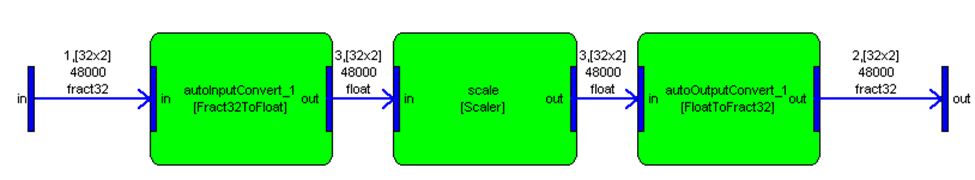
You can disable data type matching by setting:
AWE_INFO.buildControl.matchDataType=0;
When disabled, building the above system will fail. You have to manually insert the type conversion modules yourself.
Audio Weaver also automatically matches the number of channels in your system to the number of channels supported by the physical hardware. If there is a mismatch, then router modules are automatically inserted.
Consider the scaler example again. The system has 2 input and 2 output channels. If the system is built on the Audio Weaver Demo Board, which has 2 inputs and 4 outputs, then there would be a mismatch at the output: 2 channels from SYS connected to 4 channels on the target. Audio Weaver automatically corrects this by inserting a router module. After building, the system will be:
>> SYS
 = Test // Scaler match example

   autoInputConvert_1: [Fract32ToFloat]
                scale: [Scaler]
   autoOutputRouter_1: [Router]
  autoOutputConvert_1: [FloatToFract32]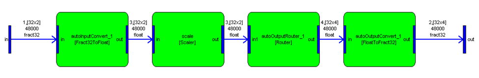
You can disable matching the number of channels by setting:
AWE_INFO.buildControl.matchNumChannels=0;
Automatic matching of data types and number of channels is a new feature introduced in Audio Weaver 2.0. Along with this change, all target platforms were standardized to have a common fract32 data type. Automatic matching simplifies the overall process of building systems, especially on a floating-point target since the required type conversion modules are automatically inserted.
target_profile.m
target_profile(SYS, FORMAT)
Computes profiling information (processor and memory utilization) for a system running in Audio Weaver. Arguments:
SYS - @awe_subsystem or @awe_module object
FORMAT - an optional string that is passed to profile_display that controls the formatting of the output data. Refer to the function profile_display.m for an explanation on how to use this argument.
The system or module SYS must be running in real-time when the profile is computed.
When called with no output arguments, the function displays detailed profiling information to the MATLAB output window. When called with an output argument:
SYS=target_profile(SYS)
The function computes the profiling information and stores it back within the .targetInfo field of each subsystem/module within the system.
For example, run the test script
SYS=agc_example;
This instantiates and builds the system SYS. Then, profile the system as:
target_profile(SYS)
Without a trailing semicolon, the following information will be displayed to the MATLAB output window:
Wire Index   Type      numChannels   blockSize   FAST_HEAP   FAST_HEAPB   SLOW_HEAP
----------   -------   -----------   ---------   ---------   ----------   ---------
1            Input     2             32          69          0            0
2            Output    2             32          69          0            0
3            Scratch   2             32          69          0            0
4            Scratch   1             32          37          0            0
5            Scratch   2             32          69          0            0
Totals       ------                              313         0            0


Total ticks per block:                   2330.7
Average ticks per block execution:       196.5 (8.43 %)
Instantaneous ticks per block execution: 204.0 (8.75 %)
Peak ticks per block execution:          8029.0 (344.48 %)


Module Name            Class            %CPU      Ticks/Process   FAST_HEAP   FAST_HEAPB   SLOW_HEAP
--------------------   --------------   -------   -------------   ---------   ----------   ---------
                       test             4.3841    102.2572        106         0            0
.autoInputConvert_1    Fract32ToFloat   0.60327   14.1237         10          0            0
.scale                 ScalerDB         0.58582   13.6902         12          0            0
.inputMeter            Meter            0.8056    18.2739         18          0            0
.agc                   AGC              1.172     26.6096         38          0            0
.agc.core              AGCCore          0.65698   14.9027         27          0            0
.agc.mult              AGCMultiplier    0.51497   11.7069         11          0            0
.outputMeter           Meter            0.69979   15.9085         18          0            0
.autoOutputConvert_1   FloatToFract32   0.51764   13.6514         10          0            0
 = test //

   autoInputConvert_1: [Fract32ToFloat]
                scale: [ScalerDB]
           inputMeter: [Meter]
                  agc: [AGC]
          outputMeter: [Meter]
  autoOutputConvert_1: [FloatToFract32]
The top section reports wire usage. The system requires a total of 6 wires and there is detailed size information for each wire. All together, the wires require 313 words of storage, and all words are 32-bit integers in Audio Weaver. The memory break down is per heap, and the wires are allocated within the memory heap named "FAST_HEAP".
The second half of the information pertains to the modules. The first line with the class name "test" is the overall system. Below is a break down by subsystem and by module. The overall system requires 4.3841% of the CPU, which in this case is a 263 MHz SHARC 21371 processor. The column "Ticks/Process" is target specific and indicates the average number of clock ticks needed to execute the function. On the SHARC, each clock tick represents 1 processor cycle, or about 3.8 nanoseconds. On the PC, each clock tick represents 100 nanoseconds. The clock tick measurements are smoothed in real-time by a first order IIR filter. The smoothing is roughly equivalent to averaging the tick counts over 100 calls to the processing function.
You can also call the profiling function with an output argument:
SYS=target_profile(SYS);
In this case, the profiling information is stored within the system structure SYS. The wire usage is contained within each of the input, output, and scratch pins. For example, to see the number of words used by the first wire in the system
>> SYS.inputPin{1}.heapSize

ans =

    69
     0
     0
Similarly, per module profiling information is contained in the .targetInfo field of each module. For example
>> SYS.agc.targetInfo

ans =

           heapSize: [3x1 double]
           heapName: {3x1 cell}
        mangledName: 'agc'
         objectAddr: []
           objectID: []
        profileTime: 5.0664
     profilePercent: 0.0739
             isSIMD: 0
               MIPS: 0.0038
    allocationOrder: []
target_get_heap_info.m
This call returns the names and sizes of all memory heaps on the target. By default, the function returns the current sizes of the heaps
>> target_get_heap_info

ans =

        10239423
        10240000
         4194304
The size of each heap is in 32-bit words. The function also returns the names of the heaps when called as:
>> target_get_heap_info('names')

ans =

    'FAST_HEAP'
    'FAST_HEAPB'
    'SLOW_HEAP''
When memory profiling is enabled in Audio Weaver, this call is made before and after each audio module is instantiated on the target. By comparing the memory sizes before and after instantiation, the memory requirements of each module can be determined.
target_get_classlist.m
Queries the Server to determine which audio module classes are available. When called with no return argument, the function lists out the available classes to the MATLAB output window. A partial example is shown below:
>> target_get_classlist;
472 Module Classes on Server
Class Name                 DLL Name              Class ID   Address      Num Public   Num Private
-------------------------  -------------------   --------   ----------   ----------   -----
ModuleBlockConcatenate     FrameDLL.dll          0          0x0FABB69C   0            0
ModuleBlockDelay           FrameDLL.dll          1          0x0FABB67C   3            1
ModuleBlockExtract         FrameDLL.dll          2          0x0FABB65C   2            0
ModuleBlockFlip            FrameDLL.dll          3          0x0FABB63C   0            0
ModuleCopier               FrameDLL.dll          4          0x0FABB61C   0            0
ModuleDeinterleave         FrameDLL.dll          5          0x0FABB5FC   0            0
ModuleDelay                FrameDLL.dll          6          0x0FABB5DC   4            1
ModuleDelayMsec            FrameDLL.dll          7          0x0FABB5AC   3            1
…
L=target_get_classlist;
When call with an output argument, the function returns an array of structures, one per audio class. Each structure contains the class name, DLL name, address of the class object on the target, the integer classID, and the number of public and private words in the instance structure. For example:
>> L(3)

ans =

     className: 'ModuleDelay'
       dllName: 'FrameDLL.dll'
          addr: 269748316
       classID: 3
     numPublic: 3
    numPrivate: 1
target_get_info.m
Queries the Server to determine properties of the target. The function returns a data structure with the fields shown below:
>> target_get_info

ans =

                    name: 'Native'
                 version: '1.0.0.4'
           processorType: 'Native'
          commBufferSize: 264
         isFloatingPoint: 1
        isFlashSupported: 1
                   numIn: 2
                  numOut: 2
            inputPinType: [1x1 struct]
           outputPinType: [1x1 struct]
    fundamentalBlockSize: 32
              sampleRate: 44100
               sizeofInt: 4
            profileClock: 10000000
                  isSIMD: 0
                   flags: [1x1 struct]
where numIn and numOut may vary depending on the user sound card . The fields contain the information below:
name – short string (8 characters at most) that identifies the target. 'Native' indicates that the processing is occuring on the PC.
version – version string in the form #.#.#.#.
commBufferSize – integer specifying the communication buffer size in 32-bit words.
processorType – string specifying the type of processor. Values currently supported are 'Native', 'SHARC', and 'Blackfin'.
isFloatingPoint – Boolean specifying whether the processor has true (not emulated) floating-point capabilities. This does not refer to the data type of the I/O pins which are always fract32.
isFlashSupported – Boolean specifying whether there is a flash file system on the target.
numIn, numOut – number of input and output channels.
inputPinType, outputPinType – structures returned by new_pin_type() which describe the input and output pins.
fundamentalBlockSize – underlying blockSize used by the DMA operation on the target. The blockSize of wires connected to the input or output pins must be multiples of the fundamentalBlockSize.
sampleRate – audio sample rate, in Hz.
sizeofInt – value of the C expression sizeof(int). This is used by the Server to determine structure offset addresses.
profileClock – speed of the underlying clock used for module profiling. On the PC, this equals 10 MHz. On the SHARC and Blackfin, this equals the processor's clock speed.
isSIMD – boolean specifying whether the target supports SIMD or not.
Commands Related to Audio Modules and Subsystems
add_control.m
Adds a single variable to a module's inspector. This command is described in Creating User Interfaces.
add_module.m
SYS=add_module(SYS, MOD)
Adds a module to an @awe_subsystem object. Arguments:
SYS - @awe_subsystem object to which to add the module
MOD - @awe_module object returned by one of the module constructors.
The updated system is returned as an output argument. If no output argument is supplied
add_module(SYS, MOD)
then the system object SYS is updated in the calling environment. The module appears as a field within the structure SYS and the field name is taken from the module's name, MOD.name. (The module's name is set as the first argument to the module constructor function.) The module name must be unique within the subsystem, and the add_module function checks for this. If a duplicate module name is supplied, the following error occurs
??? Error using ==> add_module
A module with that name already exists in the system
add_pin.m
M=add_pin(M, USAGE, NAME, DESCRIPTION, TYPE)
Adds a single input, output, or scratch pin to an @awe_module or @awe_subsystem object. Arguments:
M - @awe_module or @awe_subsystem object.
USAGE – a string indicating whether this is an 'input', 'output', or 'scratch' pin.
NAME – a short name, or label, that is used to identify the pin.
DESCRIPTION – a longer description that appears in the module documentation.
TYPE – a pin type structure returned by new_pin_type.
Examples of how to use this function are provided in Adding Modules. Note that the set of input pin names must be unique, as well as the set of output pin names. The add_pin function checks for this and reports the following error if this condition is violated:
??? Error using ==> add_pin
An input pin named 'in' already exists. Choose another name
awe_getstatus.m and awe_setstatus.m
These functions apply to audio modules and to subsystems that have been compiled, and exist natively on the target. In contrast, flattened subsystems do not support these calls. These functions query and change the run-time status of an audio module. Each audio module has an associated status that affects its run-time behavior:
'Active' – the audio module is running and its processing function is being called.
'Muted' – the module's output buffers are filled with zeros; the processing function is not called.
'Bypassed' – the module's inputs are copied directly to its outputs. The generic version copies the ith input pin to the ith output pin. A module may also define a custom bypass function if the generic version is not appropriate. Refer to Custom Modules Developer's Guide for further details about custom bypass functions.
'Inactive' – Nothing happens. When inactive, a module's output buffers are unchanged. Be careful when using inactive mode because the contents of the output buffers is undefined and will be propagated to downstream modules. Inactive mode is used primarily for debugging. When a module is placed in inactive mode, you may hear a periodic squeal at the block rate. This occurs when the module's output buffer is not touched and the previous contents are continuously recycled.
Some modules allow you to modify the run-time status via the inspector. The status control appears as 4 radio buttons as shown below:
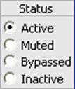
The run-time status can be changed during design time or in real-time. Note that changes occur instantly without smoothing, and audible clicks may result. To set a module's run-time status, use the command
M=awe_setstatus(M, STATUS)
where M is an @awe_module object and STATUS is a string with one of the values 'active', 'muted', 'bypassed', and 'inactive'. The function returns an object reflecting the change in status. You can also change the status of individual modules in a subsystem as:
SYS.subsystem.module=awe_setstatus(SYS.subsystem.module, STATUS);
To query a module's run-time status, use the command
STATUS=awe_getstatus(M)
Every module has an associated run-time status. A subsystem may also have a run-time status if it exists natively on the target. If the subsystem is flattened, then only the status of individual modules may be changed.
The global variable
AWE_INFO.inspectorControl.showStatusInactive
allows you to control whether the "Inactive" option is available on the inspector. By default, the variable is equal to 1 and "Inactive" is shown. If you set this to zero, then the inspector only contains the first 3 options:
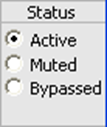
check_connections.m
STATUS=check_connections(SYS)
This functions checks the wiring within an @awe_subsystem object looking for wiring errors and completeness. This function is called automatically during the build process to ensure that the system can be properly built. Input arguments:
SYS - @awe_subsystem object.
The function returns an integer STATUS that is interpreted as:
Integer | Status |
|---|---|
-1 | There is a wiring error. |
0 | There are no wiring errors, but the wiring is not complete. There are 1 or more pins in the subsystem that are not connected. |
1 | There are no wiring errors and the wiring is complete. The system is ready to build. |
Connections within a subsystem are made by the connect.m command. Each connection is from a named source module / output pin to a named destination module / input pin. The connection.m function catches several different wiring errors:
The named source module / output pin does not exist.
The named destination module / input pin does not exist.
A module's input pin has multiple connections (illegal fan-in).
A system output pin has multiple connections (illegal fan-in).
STATUS=check_connections(SYS, FIXUP)
An optional second argument instructs the function to fix a subset of the wiring errors. If FIXUP=1, then the corrections are made. If FIXUP=0 (the default), then the corrections are not made. The function can fix the following wiring problems:
For every unconnected system input pin, the function adds a sink module.
For every unconnected module output pin, the function adds a sink module.
For every unconnected system output pin, the function adds a source module.
For every unconnected module input pin, the function adds a source module.
The source and sink modules are named "autoSource_NN" and "autoSink_NN", where NN is an integer.
Note that the function must guess at the pin type of the source modules that are added. That is because the pin type information is derived from the source module and propagated downstream. The following logic is used to derive the pin type:
The type of the first system input pin is used.
If the system has no inputs, then the type of the first output pin is used.
If the system has no inputs and no outputs, then the default pin type returned by the function new_pin_type.m. is used.
Be aware that this heuristic can often lead to mismatches in pin dimensions and sample rates. It is good practice to never have unconnected pins.
connect.m
SYS=connect(SYS, SRC, DST)
Creates a single wiring connection within an Audio Weaver subsystem. Arguments
SYS - @awe_subsystem object.
SRC – string specifying the starting pin of the connection
DST – string specifying the ending pin of the connection
The general syntax for specifying a pin is 'moduleName.pinName'. An empty module name is used to specify an input or output of the subsystem. That is, when SRC is of the form '.pinName', it specifies a subsystem input pin. Similarly, when DST is of the form '.pinName', it specifies a subsystem output pin.
The function accepts several different variations of SRC and DST to expedite wiring. If a module has only a single input or output pin, then you can leave off the '.pinName'. For example, to connect two scaler modules 'scaleA' and 'scaleB', use:
connect(SYS, 'scaleA', 'scaleB')
To connect the system input pin 'in1' to a scaler module, use
connect(SYS, '.in1', 'scaleA')
If the system has 1 input pin, then this can be shortened to
connect(SYS, '', 'scaleA');
If the source module has N output pins and the destination has N input pins, then
connect(SYS, 'sourceModule', 'destinationModule')
connects the ith output of sourceModule to the ith input of destinationModule. The function returns the updated system as an output argument. As demonstrated by the calls above, if you do not accept an output argument, then the variable SYS is updated in the calling environment.
You can also connect multiple modules in series using the syntax
connect(SYS, 'scaleA', 'scaleB', 'scaleC', 'scaleD');
This is equivalent to 3 separate calls
connect(SYS, 'scaleA', 'scaleB');
connect(SYS, 'scaleB', 'scaleC');
connect(SYS, 'scaleC', 'scaleD');
Audio Weaver also supports feedback on a block-by-block basis. The location of the feedback must be explicitly identified using a fourth argument to the connect function
SYS=connect(SYS, SRC, DST, ISFEEDBACK)
By default, ISFEEDBACK=0 and a standard feedforward connection is made. Set ISFEEDBACK=1 to indicate feedback. See Feedback for a detailed discussion of using feedback within Audio Weaver systems.
The connection function performs rudimentary error checking when called. An optional fifth input argument performs more detailed checking:
SYS=connect(SYS, SRC, DST, ISFEEDBACK, CHECK)
When CHECK=1, the function calls check_connections.m to verify the integrity of the wiring. By default, CHECK=0.
delete_connection.m
SYS=delete_connection(SYS, MOD1, PIN1, MOD2, PIN2)
Deletes a single connection within a subsystem. It essentially undoes a call to connect.m. Arguments:
SYS - @awe_subsystem object.
MOD1 – string specifying the name of the source module
PIN1 – string specifying the name of the output pin on the source module
MOD2 – string specifying the name of the destination module
PIN2 – string specifying the name of the input pin on the destination module
The function returns the updated subsystem object. This call is typically never used in practice, but is used internally by Audio Weaver when preparing a subsystem for real-time execution.
delete_module.m
SYS=delete_module(SYS, MOD)
Deletes a module from a subsystem. Arguments:
SYS - @awe_subsystem object.
MOD – string specifying the name of the module
The function deletes the module from the subsystem and also deletes any connections to the module. The function returns the updated subsystem object SYS. This function is typically not used in practice, but is used internally by some of the other Audio Weaver functions (flattening, in particular).
delete_module(SYS, MOD)
If no output argument is accepted, then the function updates the object SYS in the calling environment.
draw.m
draw(SYS)
draw(MODULE)
Draws a graphical representation of a module or subsystem in a MATLAB figure window. This is useful when developing and debugging subsystems. For example, to draw an agc_multiplier.m module, issue the commands:
>> M=agc_multiplier_module('mult');
>> draw(M)
The following drawing appears in a MATLAB figure window:
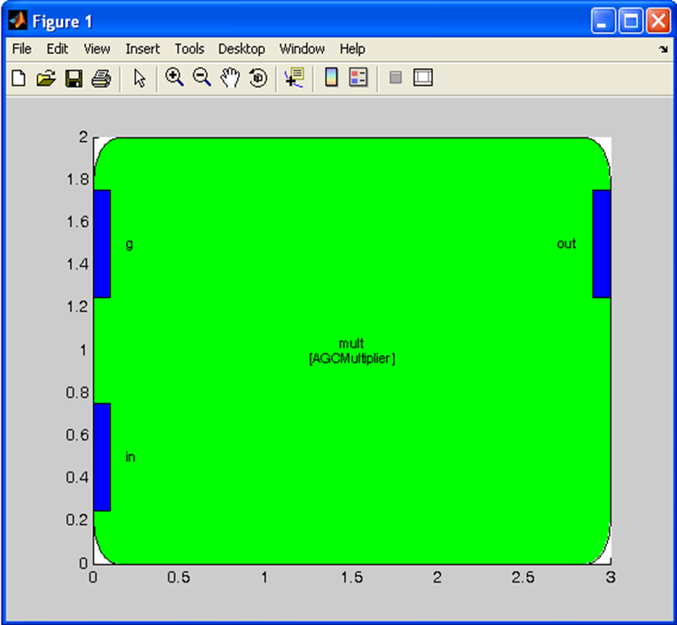
The module name and class name (in brackets) are shown in the center of the figure. The input and output pins are indicated by filled rectangles and identified by pin labels.
When you draw a subsystem, the figure window shows the individual modules as well as connections. For example, if you instantiate and draw a limiter subsystem,
>> SYS=limiter_module('lim', 96);
>> draw(SYS)
the figure shown below is drawn:
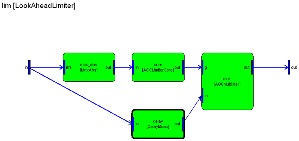
The figure contains the following information:
Input and output pins are shown on the left and right edges, respectively.
Internal modules are drawn together with current parameter settings.
Internal connections are drawn.
The top left corner indicates subsystem name [class name].
A toolbar on the figure window allows you to adjust the display:
Button | Function |
|---|---|
 | Zoom in |
 | Zoom out |
 | Scroll the display |
 | Display wire information (toggle) |
 | Display module variables (toggle) |
 | Display pin names (toggle) |
 | Refresh the drawing |
All of the tools labeled "toggle" are global and apply to subsequent drawings. The state of the toggle buttons is stored in the global variable:
>> AWE_INFO.drawControl

ans =

    showVariables: 0
    showWireTypes: 0
     showPinNames: 1
When wire information is shown, each connection in the diagram is labeled with its wire index, block size, number of channels, and sample rate. The notation used is
Wire index,[blockSize numChannels]
sampleRate
dataType
Displaying wire information for the previous system shows:
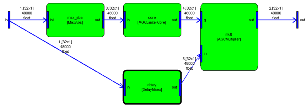
The wire index identifies a wire within the subsystem. Wires are always indexed in the same manner: wire(s) attached to input pins (#1), wire(s) attached to output pins (#2), and intermediate scratch wires (#3, and #4). The wire indexes shown are local to the subsystem. That is, within every subsystem, the wires are indexed as input wires, output wires, and then scratch wires.
Some modules may utilize the same wire for both input and output. This "straight across" wire buffer allocation is specified within the module's constructor function. Further details are found in Custom Modules Developer's Guide (No modules in the limiter_example.m have straight across wiring).
A subsystem drawing also gives insight into the execution order of the internal modules. The modules execute from left to right and top to bottom. For example, after the limter_example.m builds, the subsystem contains the modules:
>> SYS=limiter_example;
>> SYS
 = test //

   autoInputConvert_1: [Fract32ToFloat]
                scale: [ScalerDB]
                  lim: [LookAheadLimiter]
           firstMeter: [Meter]
          secondMeter: [Meter]
   autoOutputRouter_1: [Router]
autoOutputConvert_1: [FloatToFract32]
The modules are executed in the order listed. First 'scale' executes, then 'lim', and so forth. Looking at the subsystem drawing, we see this same ordering enforced.
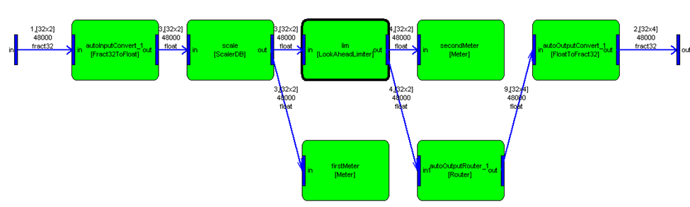
Limiter Example Figure Drawing
Audio Weaver tries its best to make legible drawings based on the order of execution of the modules. In some cases, the drawings are difficult to understand because of overlapping wires and modules. Consider the example below taken from echo_subsystem_example.m. The figure has a feedback wire – from the output of EchoHighCut to the first input of EchoFeedbackScaleAdd. Also, the output of the system is taken from EchoDelay. Both of these connections are not at all clear from the drawing.
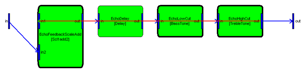
Audio Weaver allows you to nudge the location of modules and system pins to improve the drawings. Modules and pins have a .drawInfo.nudge field which specifies a drawing offset. By default, the nudge values are empty indicating that the items will be drawn at their automatically computed positions. Within the subsystem constructor (echo_subsystem.m), the following 2 lines are added:
SYS.outputPin{1}.drawInfo.nudge=[0 1];
SYS.EchoHighCut.drawInfo.nudge=[0 -1];
The nudge values are 1x2 arrays with X and Y offsets. A positive X nudge value moves the item to the right; a positive Y nudge value moves the item up. With these changes, the drawing now appears as shown below. The output pin has been raised and the EchoHighCut module lowered. The connections are clear.
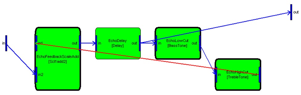
When subsystems are drawn using the draw.m command, the modules are color coded according to their status:
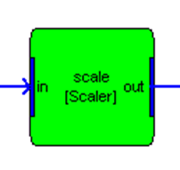 |
|
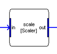 | Muted = White |
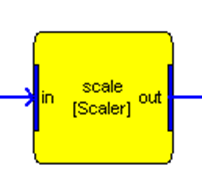 | Bypassed = Yellow |
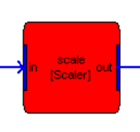 | Inactive = Red |
If you make a change to the module status using either an inspector or programmatically from MATLAB using the awe_setstatus.m command, then the drawing in a figure window will not be automatically updated. Instead, you need to manually refresh the window using the toolbar button or right-clicking on an empty part of the figure window and selecting Redraw.
findconnection.m
C=findconnection(SYS, MOD1, PIN1, MOD2, PIN2)
Locates connections within a subsystem and returns a cell array describing the individual connections. Arguments:
SYS - @awe_subsystem object.
MOD1 – string specifying the name of the source module. Set this to the empty string to specify an input of the system.
PIN1 – name of the source pin.
MOD2 – name of the destination module. Set this to the empty string to specify an output of the system.
PIN2 – name of the destination pin.
The function returns a cell array of structures. There is one cell array entry per connection and each structure contains the fields:
.srcModName – name of the source module. An empty string specifies an input to the system.
.srcPinName – name of the pin on the source module.
.dstModName – name of the destination module. Am empty string specifies an output of the system.
.dstPinName – name of the pin on the destination module.
The real power of this function comes from its ability to support wild cards. Use the string '*' to specify any module or pin. For example, consider the Limiter Example Figure Drawing.
To determine what modules are connected to the output of the "scale" module, use:
>> C=findconnection(SYS, 'scale', '*', '*', '*')

C =

    [1x1 struct]    [1x1 struct]
The returned cell array C contains two entries. Looking at each entry in detail we see:
>> C{1}

ans =

    srcModName: 'scale'
    srcPinName: 'out'
    dstModName: 'firstMeter'
    dstPinName: 'in'
    isFeedback: 0

>> C{2}

ans =

    srcModName: 'scale'
    srcPinName: 'out'
    dstModName: 'lim'
    dstPinName: 'in'
    isFeedback: 0
Thus, there are two connections from "scale" to "firstMeter" and from "scale" to "lim".
There are no connections from the input of the system directly to the output of the system. The result is an empty cell array.
findconnectiondst.m
[MODINDEX, PININDEX]=findconnectiondst(SYS, MOD, PINNAME)
Locates specific pins in a subsystem that can be used as the destination of a connection. The pin is returned as a module index and a pin index. This function is used to automate wire and routing operations within a subsystem. Arguments:
SYS - @awe_subsystem object.
MOD – string specifying the name of the module. An empty string specifies an output of the system.
PINNAME – string specifying the name of the destination pin.
The function locates the named module within the subsystem and returns its index as the first output argument MODINDEX. MODINEX=0 indicates that MOD specifies a subsystem output. MODINDEX=-1 indicates that a module named MOD was not found. Similarly, PININDEX specifies the index of the destination pin (a source pin on a module or a system output pin). INDEX=-1 indicates that the index was not found.
As an example, refer back to the system created by the script limiter_example.m shown in the Limiter Example Figure Drawing. Let's locate the input pin "in" on the "lim" module. This is the destination of a connection:
>> [MODINDEX, PININDEX]=findconnectiondst(SYS, 'lim', 'in')

MODINDEX =

     3


PININDEX =

     1
Thus, we are connected to pin 1 on module 3 within the subsystem. Looking inside, we find:
>> SYS.module{3}
lim = LookAheadLimiter // Multi-channel soft knee limiter with look ahead

  max_abs: [MaxAbs]
     core: [AGCLimiterCore]
    delay: [DelayMsec]
     mult: [AGCMultiplier]

>> SYS.module{3}.inputPin{1}

ans =

              type: [1x1 struct]
             usage: 'input'
              name: 'in'
       description: 'Audio Input'
    referenceCount: 0
        isFeedback: 0
             coord: [NaN NaN]
         wireIndex: 3
findconnectionsrc.m
[MODINDEX, PININDEX]=findconnectionsrc(SYS, MOD, PINNAME)
This function is similar to findconnectiondst.m except that it locates pins within a subsystem that can serve as the source, or starting point, of a connection. This includes any system input pins or module output pins. Arguments:
SYS - @awe_subsystem object.
MOD – string specifying the name of the module. An empty string specifies a system input pin.
PINNAME – name of the pin on the module or subsystem.
As an example, refer back to system created by the script limiter_example.m shown in the Limiter Example Figure Drawing. To locate the output pin "out" of the module "scale" use
>> [MODINDEX, PININDEX]=findconnectionsrc(SYS, 'scale', 'out')

MODINDEX =

     2


PININDEX =

     1
This points to the module at index 2:
>> SYS.module{2}
scale = ScalerDB // DB multichannel scaler

  gainDB: 30        [dB] // Gain in DB
And the first output pin on this module:
>> SYS.module{2}.outputPin{1}

ans =

              type: [1x1 struct]
             usage: 'output'
              name: 'out'
       description: 'audio output'
    referenceCount: 0
        isFeedback: 0
             coord: [NaN NaN]
         wireIndex: 3
findmodule.m
MODINDEX=findmodule(SYS, MOD)
Locates a named module within an Audio Weaver subsystem. The function returns the index of the module. Arguments:
SYS - @awe_subsystem object.
MOD – string name of the subsystem.
The function returns MODINDEX, the index of the named module within the .module{} cell array. If MODINDEX=-1, then the module was not found. Set MOD equal to the empty string to specify the overall subsystem. In this case the function will return MODINDEX=0.
As an example, refer back to system created by the script limiter_example.m shown in the Limiter Example Figure Drawing. To determine the index of the module "secondMeter", use the call
>> index=findmodule(SYS, 'secondMeter')

index =

     5
Peering into the system, the 5th module is
>> SYS.module{index}
secondMeter = Meter // Peak and RMS meter module

meterType: 0          // Operating module of the meter
      value: [1.0018
              1.00951]
findpin.m
INDEX=findpin(M, IO, PIN)
Searches a module or subsystem and returns the index of a named pin. Arguments:
M - @awe_module or @awe_subsystem object.
IO – a string set to either 'input' or 'output'. This specifies whether the input or output pins should be searched.
PIN – string name of the pin to locate.
The function returns the index of the named pin. If the named pin is not found, the function returns -1.
For example, consider the limiter_example.m shown in Limiter Example Figure Drawing. The agc_multiplier module has two input pins as shown below:
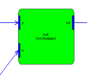
To locate the index of the input pin 'in', issue the command:
>> index=findpin(SYS.lim.mult, 'input', 'in')

index =

     2
flatten.m
SYS=flatten(SYS)
This function operates on subsystems and promotes all internal modules to the upper level. It ends up eliminating hierarchy and returning a “flattened” subsystem. Arguments:
SYS - @awe_subsystem object.
The flatten.m function traverses a subsystem and searches for subsystems with virtual hierarchy. When a virtual subsystem is found, all of the modules in the subsystem are promoted one level to the upper system, reconnected, and finally the original virtual subsystem is deleted. This process repeats until all virtual subsystems have been flattened.
As an example, consider the subsystem created by the test script limiter_example shown in the Limiter Example Figure Drawing. The system shown is the one prior to flattening. The actual system running on the target is
draw(flatten(SYS))
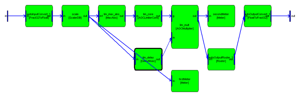
What is happening here? Well, the limiter subsystem, SYS.lim, uses virtual hierarchy. The limiter contains the 4 modules shown below:
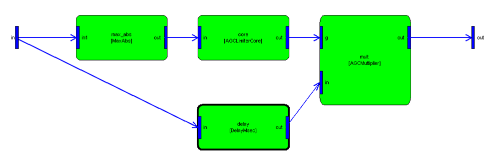
During the build process, all 4 of the modules comprising the limiter subsystem are promoted one level in the hierarchy and rewired. The delay module, lim_delay, however, is not flattened out. It uses full hierarchy and the target processor contains a module of class DelayMsec.
The standard Audio Weaver build.m command performs flattening as part of the overall build process.
Examining the last figure closely, one sees that the names of the modules from the limiter subsystem have been mangled. That is, the names have been prepended with the name of the original subsystem. This can also be seen in the flattened system shown below:
>> flatten(SYS)
 = test //

   autoInputConvert_1: [Fract32ToFloat]
                scale: [ScalerDB]
          lim_max_abs: [MaxAbs]
             lim_core: [AGCLimiterCore]
            lim_delay: [DelayMsec]
             lim_mult: [AGCMultiplier]
           firstMeter: [Meter]
          secondMeter: [Meter]
   autoOutputRouter_1: [Router]
autoOutputConvert_1: [FloatToFract32]
Typically, the user does not need to be concerned with flattening – it occurs automatically behind the scenes. The flattened system is hidden and the user continues to interact with the original hierarchical system. However, the flattened system is in fact instantiated on the target. The hierarchical system SYS maintains the mapping from the hierarchical system to the flattened system. Making a change to the hierarchical system causes a corresponding change in the flattened system. The mapping is maintained within the .targetInfo.mangledName field of each module. For example, the mangled name of the limiter core module on the target is:
>> SYS.lim.core.targetInfo.mangledName

ans =

lim_core
get_variable.m and set_variable.m
Extract and assign individual awe_variable objects. These functions apply to audio modules and subsystems. These functions are needed at times, because of the object oriented nature of the Audio Weaver MATLAB functions. When accessing a variable "var" within a module "M", as in:
M.var
Audio Weaver returns the value of the variable, not the variable object itself. If you wish to gain access to the actual variable object, use the call:
V=get_variable(M, NAME)
where
M – the @awe_module object.
NAME – a string specifying the name of the variable.
The function returns an awe_variable object. For example, the following code gets the underlying awe_variable object for the "gain" variable of a smoothed scaler module:
M=scaler_smoothed_module('scaler');
V=get_variable(M, 'gain');
Similary, the set_variable.m command can be used to overwrite an existing variable to a given awe_variable object. The term "overwrite" is used because the variable must already exist within the audio module. The syntax for this command is:
M=set_variable(M, NAME, VAR)
where
M – the @awe_module object.
NAME – a string specifying the name of the variable.
VAR - awe_variable object.
The get_variable.m and set_variable.m functions are typically not used in practice. You can always access the internal fields of a awe_variable object even when it is part of an audio module. For example, to access the "range" field of the variable "gain", use:
range=M.gain.range;
4.5.17. isfield.m
This function is similar to the standard isfield function within MATLAB applied to @awe_module and @awe_subsystem objects. The function determines if a module or subsystem has a specified variable. The syntax is:
BOOL = isfield(M, FIELDNAME)
where
M – the @awe_module object.
FIELDNAME – a string specifying the name of a variable.
The function returns 1 if the module M has a field named FIELDNAME. Otherwise, the function returns 0. Note, the function only queries variables that are part of the audio module or subsystem and not any of the private object fields.
module_count.m
COUNT=module_count(SYS)
Returns the number of modules at the top level of a subsystem.
COUNT=module_count(SYS, 1)
An optional second argument allows you to specify that the count should be recursive. In this case, the function returns the total number of modules within the entire subsystem including any modules within subsystems. For example, the system created by limiter_example.m contains 6 modules at the top level:
>> module_count(SYS)

ans =

     7
and a total of 9 modules when modules within the LookAheadLimiter subsystem are counted:
>> module_count(SYS, 1)

ans =

     10
new_pin_type.m
Creates a structure that represents a pin on an audio module or subsystem. A pin contains information about the current number of channels, block size, sample rate, data type, and complexity, as well as the allowable range for each of these items. Refer to the discussion in Section 4.1.3.
process.m
[SYS, WIRE_OUT]=process(SYS, WIRE_IN, NUMBLOCKS)
Sends audio data block-by-block through an audio system in non-real-time. This function is primarily used for regression testing. Arguments:
SYS - @awe_subsystem object. This must be a top-level system.
WIRE_IN – cell array of input wire data. The data for each input pin is represented by a matrix of dimension [L x blockSize numChannels], where L is the number of blocks. Note that each channel of data is in a separate column of the matrix. WIRE_IN contains a cell array of matrices.
NUMBLOCKS = the number of audio blocks in the simulation, equal to the variable L above.
Note that each input pin must contain the same number of blocks. If this condition is violated, the function will return an error. (You may be wondering why NUMBLOCKS needs to be specified as an argument; can't the function determine this from the size of the input pin data? The reason is that some modules, such as the sine wave generator, do not have any input pins and therefore the number of blocks needs to be explicitly stated.)
The function returns the updated system object SYS (state variables are updated) and a cell array of output wire information. WIRE_OUT has the same form as WIRE_IN, with one cell array entry per output pin. For each output wire, there is a matrix of data of size [L x blockSize numChannels].
When the system is built using a MATLAB target system, all processing occurs natively within MATLAB. When the system is built for the Audio Server, then the processing happens on the target processor (PC or SHARC) itself. Module regression tests generally rely on the process.m function. (The approach used by DSP Concepts to validate the audio module library is to perform the processing twice; once in MATLAB, and a second time on the target processor. The outputs of both implementations are then compared to detect errors. The MATLAB implementations of the audio module processing functions are not provided in Audio Weaver Developer or Designer; they are used internally by DSP Concepts. The MATLAB target system is provided to allow you to test your own custom audio modules.)
The example shown below is contained within the script file process_example.m. The script demonstrates how to send data through an Audio Weaver module and then plots the output results.
We start by creating a MATLAB target system with 1 input, 1 output, and operating at a sample rate of 44.1 kHz:
% Create a subsystem with a single second_order_filter module.
blockSize=64;
SR=44100;

SYS=matlab_target_system('test', 'Process.m example system');

add_pin(SYS, 'input', 'in', 'Audio input', new_pin_type(1, blockSize, SR));
add_pin(SYS, 'output', 'out', 'Audio output', new_pin_type(1, blockSize, SR));

add_module(SYS, second_order_filter_module('sof'));

connect(SYS, '', 'sof');
connect(SYS, 'sof', '');
The second order filter module is configured to be a peak filter with Q=1 and 12 dB of gain at 2 kHz:
SYS.sof.filterType=12;

SYS.sof.freq=2000;
SYS.sof.Q=1;
SYS.sof.gain=12;
Configure the build process to disable automatic data type matching. This prevents fract32_to_float and float_to_fract32 modules from being inserted and allows us to send floating-point data directly to the module. Then build the system:
global AWE_INFO;
global AWE_INFO;
AWE_INFO.buildControl.matchDataType=0;
SYS=build(SYS);
Since this system operates natively in MATLAB, no commands are sent to the Audio Server.
A linear chirp signal with duration 0.25 seconds is created in MATLAB. The length of the signal is rounded up to the nearest 64 sample block size.
duration=0.25;
L=SR*duration;

numBlocks=ceil(L/blockSize);

L=numBlocks*blockSize;

n=0:(L-1);
n=n(:);
T=n/SR;

x=chirp(T, 0, duration, SR/4);
The input wire cell array is created, the data passed through the system, and the resulting data extracted from the first output wire:
WIRE_IN={x};
[SYS, WIRE_OUT]=process(SYS, WIRE_IN, numBlocks);
y=WIRE_OUT{1};
Lastly, the results are plotted.
subplot(211);
plot(x);
set(gca,'YLim', [-5 5]);
title('Input data');

subplot(212);
plot(y);
set(gca,'YLim', [-5 5]);
title('Output data');
The resulting figure is shown below. The top subfigure shows the input to the system. Note that it has an amplitude of +/-1dB. The bottom subfigure shows the output of the system. Note that it has a peak gain of 4, which equals 12 dB, at 2kHz:
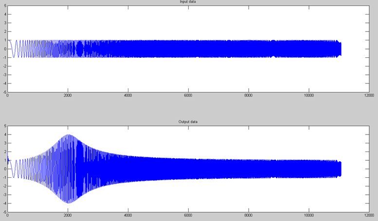
Example of the output generated by the process.m function. The top figure is the input signal, a linear chirp. The bottom figure is the output of the second order filter module. The filter is configured as a peaking filter centered at 2kHz.
readd_module.m
SYS=readd_module(SYS, HNAME, OLDNAME, NEWNAME, ARGS)
Updates a module by recreating it using different sets of instantiation arguments. Arguments:
SYS - @awe_subsystem object.
HNAME - hierarchical name of the subsystem containing the module. To change a module in the top-level system, set HNAME=''.
OLDNAME - existing name of the module.
NEWNAME - new name for the module.
ARGS - cell array of input arguments. These are passed to the module instantiation function following NEWNAME.
update.m
Explicitly calls the update (or set) function associated with a module. This function is used only in a few instances; typically all updates happen automatically. For example, if you instantiate a scaler_smoothed_module.m, and then change the smoothing time:
M=scaler_smoothed_module('scaler');
M.smoothingTime=15;
Audio Weaver will automatically call the function scaler_smoothed_set. (This function is an internal function defined within scaler_smoothed_module.m). This function computes the smoothing coefficient based on the sample rate and smoothing time.
The only time that the update function is called explicitly is at the end of the module constructor function. The update function is called to initialize any derived parameters to default values.
A module's set function is specified as a function pointer within the private fields of the class object. To see the update function (or even to override it), access it as:
>> M.setFunc

ans =

    @scaler_smoothed_set
Displaying Module Documentation
Audio Weaver modules include on-line help in HTML format. For example, to see the generated help for the Hilbert transform module, type
awe_help hilbert_subsystem
at the MATLAB command line. Behind the scenes, MATLAB checks if documentation already exists for the module. Since the hilbert_module.m function exists in the directory
<AWE>\Modules\AdvancedAudioFloat32\Subsystems
it checks if the file
<AWE>\Modules\AdvancedAudioFloat32\Doc\Hilbert.html
exists. The name "Hilbert.html" is based on the module's class name. If the file exists, it is opened and displayed in the MATLAB HTML browser. If it doesn't exist, then the documentation is generated on the fly using Microsoft Word and then saved in HTML format. The process of generating new documentation is quite involved and can take 20 to 30 seconds to complete.
If the HTML file exists, you can force it to be rebuilt using the optional argument shown below:
awe_help hilbert_module --rebuild
The process of documenting modules is detailed in the Audio Weaver Module Developers Guide.
Advanced System Design Features
This section discusses advanced system design features including multirate processing and feedback.
Multirate Processing
Audio Weaver supports multirate processing through the use of decimator and interpolator modules. There are two restrictions that must be observed:
The block size must always be an integer number of samples.
All audio modules execute at the same rate in time.
This second restriction is equivalent to requiring that blockSize/sampleRate be equal throughout the audio layout.
For example, consider a system operating at a 32 sample block size with a sample rate of 48 kHz. If this is interpolated by a factor of 3, then the resulting audio signal will have a block size of 96 samples and a sample rate of 144 kHz. Note that in both cases the time duration of each block equals 32/48000 = 96/144000 = 2/3 msec. Now continue with a factor of 8 decimator. The block size is then 12 samples and the sample rate is 18 kHz; the time duration of each block remains 2/3 msec.
Each audio buffer is marked with its block size and sample rate. As a result, each audio module within the signal chain can locally determine and utilize this information to compute filter or smoothing coefficients.
In floating-point systems, there are 4 multirate modules that provide decimation or interpolation:
downsampler_module.m – Downsampler or decimator. It keeps 1 out of every D samples; no filtering involved.
fir_decimator_module.m – Combined FIR filter and decimator module. The processing is implemented using an efficient polyphase realization.
The output block size equals the input block size divided by D. The output sample rate equals the input sample rate divided by D. In all cases, the decimation factor D must evenly divide the input block size so that the output block size is an integer. This requirement is checked by the module's prebuild function.
upsampler_module.m – Upsampler or interpolator. The module inserts L-1 zeros between each sample.
fir_interpolator_module.m – Combined upsampler and FIR filter. The processing is implemented using an efficient polyphase realization.
There are no restrictions placed on the upsampling factor L. The output block size equals the input block size times L. The output sample rate equals the input sample rate times L.
There are equivalent modules for fixed-point processing:
downsampler_module.m (the same module supports float and fract32 data types).
fir_decimator_fract32_module.m
upsampler_module.m (the same module supports float and fract32 data types).
fir_interpolator_fract32_module.m
Multiple Audio Processing Threads
In the previous section on multirate processing all of the blocks have the same time duration and modules execute sequentially in the same thread. In some cases, you would like the audio processing to have multiple block sizes and each block size operates in a different thread. For example, the main audio processing may occur with a 32-sample block size while a separate measurement thread operates at a 128-sample block size. If the same rate is 32 kHz, then the main audio processing occurs every 1 msec while the measurement process occurs every 4 msec. The large block processing occurs in a separate lower priority interrupt and is periodically interrupted by the higher priority 32-sample block processing. This is illustrated in the figure below:
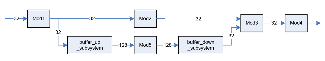
The interface between the 32- and 128-sample block processing is accomplished by two modules:
buffer_up_subsystem.m – handles the interface between smaller and larger block size processing (e.g., 32 to 128)
buffer_down_subsystem.m – handles the interface between larger and smaller block size processing (e.g., 128 to 32)
The arguments to buffer_up_subsystem are:
buffer_up_subsystem(NAME, OUTBLOCKSIZE)
The second argument specifies the output blockSize. If OUTBLOCKSIZE is a positive number, then the output blockSize equals OUTBLOCKSIZE. If OUTBLOCKSIZE is a negative number, then the output blockSize equals the input blockSize times (-OUTBLOCKSIZE). For example, if you set OUTBLOCKSIZE = -4 then the output blockSize will always be 4 times the input blockSize.
The arguments to buffer_down_subsystem.m are similar:
buffer_down_subsystem(NAME, OUTBLOCKSIZE)
However if OUTBLOCKSIZE is negative, then it is used as a divider. For example, if OUTBLOCKSIZE = -4, then the output blockSize will be set to ¼ of the input blockSize.
Converting between different block sizes requires some internal buffering. The rule of thumb to keep in mind is that the overall latency equals twice the larger block size. If you want to maintain time alignment throughout your audio processing, you have to insert a compensating delay:
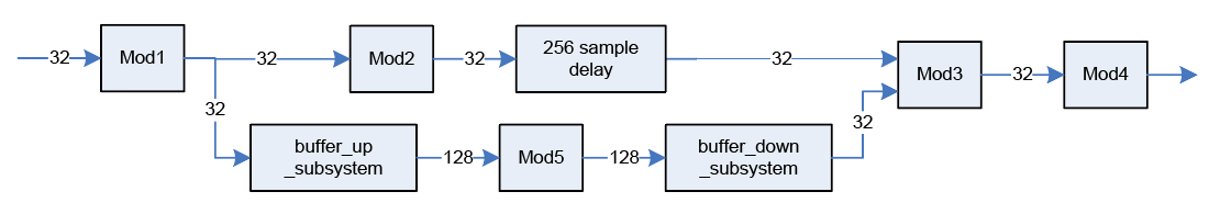
We now go into more detail to describe how multiple audio processing threads are implemented in Audio Weaver. The figure below shows processor activity when audio is processed in 32- and 128-sample blocks (1 msec and 4 msec).
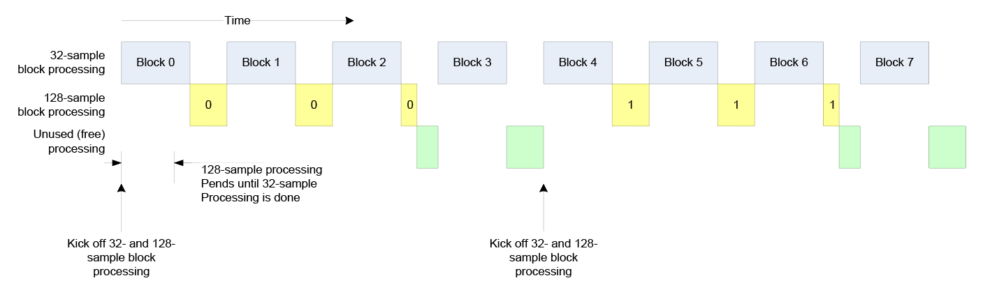
The top line of blue blocks indicates when 32-sample audio processing is active. This happens at regular intervals and since this is the smallest block processing (and thus the highest priority), the 32-sample processing always runs to completion. The blocks are sequentially numbered from 0 to 7. The second line of yellow blocks indicates when the 128 sample block processing is active. Block 0 of the 128-sample processing actually starts at the same time as block 0 of the 32-sample processing. However, since the 32-sample block processing is higher priority, the 128-sample thread pends until the 32-sample processing is complete. Once the 32-sample processing is done, the 128-sample processing begins. Block 0 of the 128-sample processing takes some time to complete and during this time it is interrupted by the high priority 32-sample block processing. That is why block 0 of the 128-sample processing is divided into 3 different segments. Block 0 of the 128-sample processing completes and this leaves some unused processing shown in blue. The entire process repeats every 128 samples.
An important question to consider is which samples are available at each time slice for processing. This is illustrated below. The diagram has been slightly simplified to make it easier to follow. Although the 128-sample block processing is shown continuously processing, it is in fact interrupted by the 32-sample block processing.
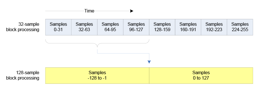
The main thing to note is that there is a 128 sample delay between the 32- and the 128-sample block processing. This delay occurs because we have to wait until we have a complete 128-sample block before kicking off the processing. This delay requires buffering and Audio Weaver provides two subsystems which serve as interfaces between different sized block processing:
Internally, each subsystem contains a fifo_in_module.m and a fifo_out_module.m. These FIFO’s provide the buffering needed to connect the two clock domains. Expanding the subsystems we see:
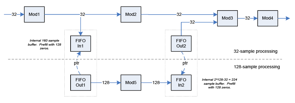
The fifo_in_module copies data from its input pin to an internal circular buffer. The fifo_out_module has a pointer variable which is initialized (in buffer_up_subsystem.m) to point to the fifo_in_module.m. When the fifo_out_module.m is executed, it copies data from the fifo_in_module to its output pin. In the example above, the FIFO Out1 module copies data out in blocks of 128 samples while the FIFO Out2 module copies data out in 32-sample blocks. Each fifo_in_module is also pre-filled with a number of zero samples.
Let’s look closely at the behavior of this system. The execution order for modules in the 32-sample domain is:
Mod1, FIFO In1, Mod2, FIFO Out2, Mod3, Mod4
The execution order for modules in the 128-sample domain is:
FIFO Out1, Mod5, FIFO In2
The figure below shows how the processing progresses block-by-block. The focus is on what data is contained within each FIFO buffer. The data enters the FIFO on the right hand side and then exits on the left hand side. Each cell corresponds to 32-samples. “Z” indicates that the cell has been prefilled with zeros. “---“ indicates that there is no data in the cell. That is, the FIFO is not full. And finally, numbers in a cell indicate specific sample indices. Negative values refer to numbers from the previous block. The yellow blocks correspond to the initial prefilling. The green blocks correspond to the 32 sample processing and the blue blocks correspond to the 128 sample processing.
It can be seen that prefilling is important because some of the fifo_out_module’s are asked to output data before the input is available. You can also ascertain where the buffer sizes came from. Each FIFO buffer becomes full sometime during the processing cycle. And finally, keep an eye on the 0 to 31 block of input samples. It takes quite a bit of time to work its way through the system. It is not until the final set of green boxes that the 0 to 31 samples are output. In fact, the latency through the two buffering stages is exactly 128 samples; twice the larger block size. This relationship holds for other block sizes as well.
There are certain assumptions built into the helow figure. First, the example assumes that all of the 128 sample block processing completes before the second block of 32-samples is processed. This is not a hard requirement since large block processing is only useful if the processing can extend over multiple smaller 32-sample blocks.
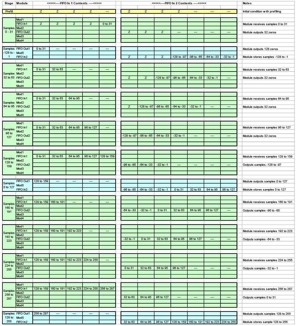
Time evolution of the FIFO buffers when 32- and 128-sample block sizes are mixed. This shows the case when the 128-sample processing completes before the next block of 32-samples is processed.
The below figure shows how the processing evolves if the 128 sample block size processing takes much longer to complete. You’ll note that the data in FIFO In2 arrives just in time to fullfill the request to output 32-samples. The overall latency remains at 256 samples.
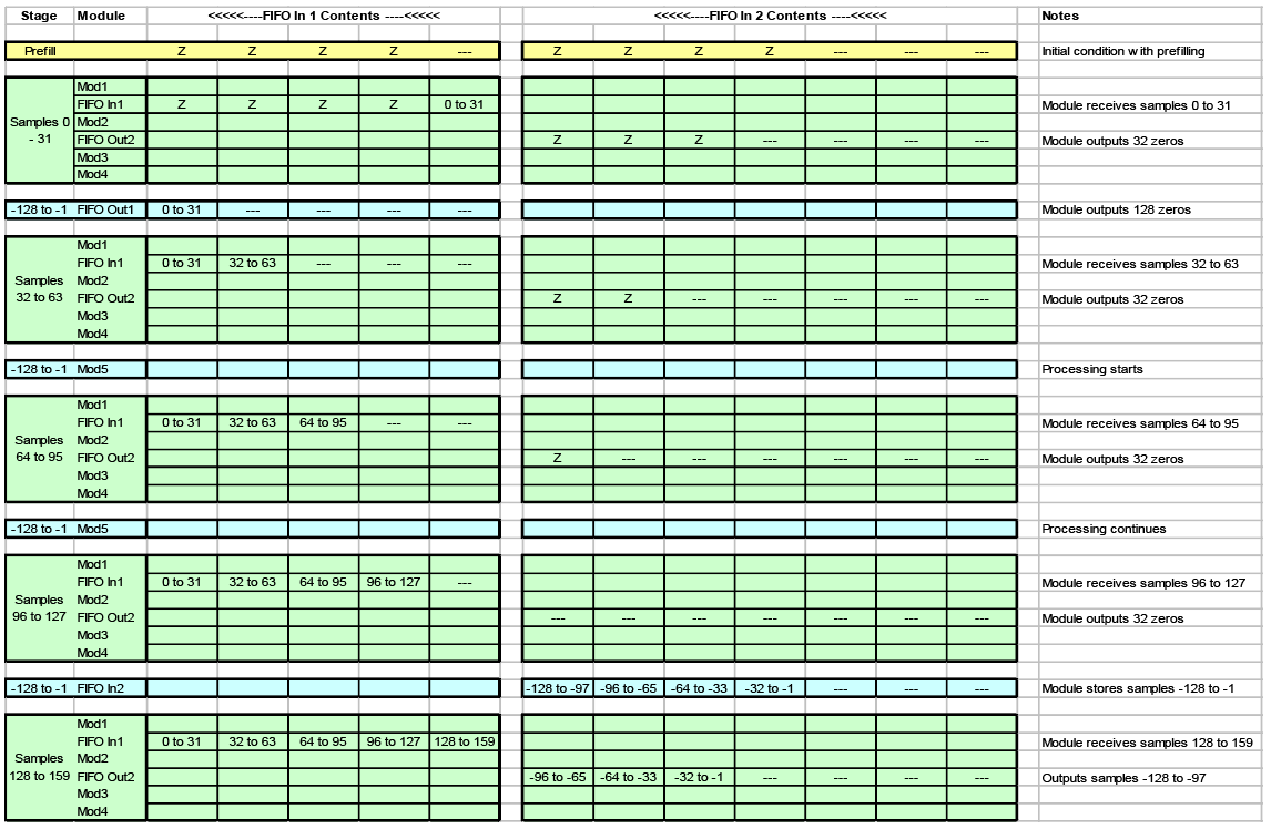
Time evolution of the FIFO buffers when 32- and 128-sample block sizes are mixed. This shows the case when the 128-sample processing takes a long time and completes just before the 4th block of 32-samples is processed.
A related module is the rebuffer_module.m which buffers up data into overlapping blocks.
Feedback
Feedback is a key building block for audio algorithms and is frequently used in reverberation and dynamics processors. There are a number of issues to keep in mind when using feedback in Audio Weaver. This section describes how to add feedback to a system and gives a complete example of a subsystem incorporating feedback.
Feedback and Feedfoward Connections
Most connections in Audio Weaver are feedforward. That is, the output of a module (or the input of the subsystem) serves as input for subsequent modules. Audio data flows from left to right in the signal flow diagram.
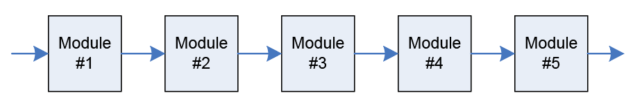
System containing only feedfoward connections.
Feedback occurs when an audio signal travels from right to left in the signal flow diagram. The output of a module serves as input to an earlier occuring module in the system.
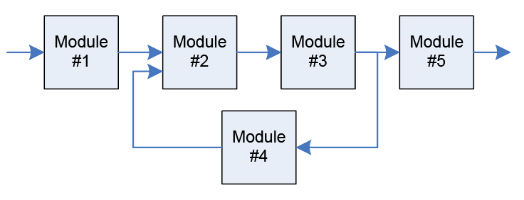
System containing both feedfoward and feedback connections.
Systems with feedback can only be realized when there is a delay in the feedback path. Audio Weaver automatically inserts the delay for you, and the delay occurs on a block-by-block basis. If you need less delay you'll need to reduce the block size of the system.
Point-to-point connections in Audio Weaver are specified via the connect.m function described in connect.m The connect.m command has an optional fourth argument which is used to indicate feedback.
SYS=connect(SYS, SRC, DST, ISFEEDBACK)
When you make a feedback connection, you explicitly identify the location at which the feedback and the associated delay occur. Recall that connections between modules correspond to buffers of data. The routing algorithm allocates buffers as needed and attempts to reuse buffers whenever possible in order to conserve memory. When feedback occurs, a new wire buffer is allocated and never reused. This wire buffer holds the delayed data and implements the delay of 1 block.
Behavior Depends on the Feedback Location
The location of the feedback connection affects the behavior of the system. For example, suppose that the feedback connection in the previous diagram occurs between modules 4 and 2. Then the delay will be inserted at that location:
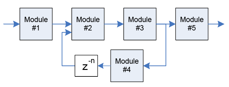
Specifying the connection between module 4 and module 2 as feedback inserts the delay at the location shown.
where n = blockSize. Note that the delay occurs as a result of the buffer management. A delay module is not inserted at this location. The modules in the subsystem will execute in the following order:
Module #1
Module #2
Module #3
Module #4
Module #5
Conceptually, the diagram can be redrawn as shown below since there is only 1 feedback connection:
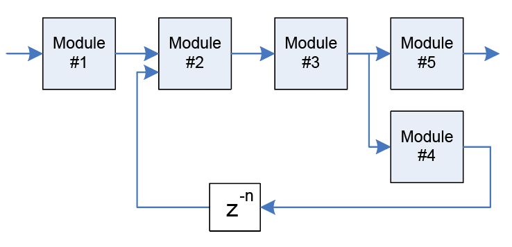
Redrawing the figure to indicate a single feedback signal.
Alternatively, suppose that the feedback occurs between modules 3 and 4. Module 3 will then have both a feedforward and a feedback connection. If a feedback buffer is allocated for the output of module 3, then the input to module 5 will also be delayed – but this is not the desired behavior. To deal with this special case topology, Audio Weaver automatically inserts a copier module into the system at the output of module 3. The feedback connection is isolated from the feedfoward connection by the copier. The system is then as shown below:
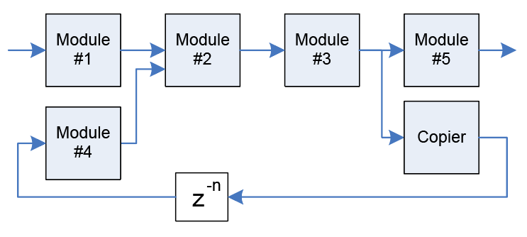
Resulting signal flow when the feedback point is specified between module 3 and module 4. A copier module is automatically inserted to isolate the feedfoward and feedback connections at the output of module 3.
The modules in the system will execute in the following order:
Module #1
Module #4
Module #2
Module #3
Module #5
Copier Module
Although the redrawn systems are structurally different due to differences in the feedback location, the outputs will be identical as long as module 4 is time invariant.
Feedback connections cannot be made to the input or output of a subsystem; they must be internal to a subsystem. This is a logical problem with these types of connections. What does it mean for system input or output to be feedback? The connect.m function checks for this.
Explicitly Specifying Feedback Pin Information
There is one final complexity associated with using feedback. Recall that the routing algorithm propagates pin information throughout the system. The algorithm starts at the input pins and then propagates the pin type (numChannels, blockSize, sampleRate, and dataType) from module to module. If feedback occurs in a system, you must explicitly set the pinType at the source of the feedback wire; it is impossible for Audio Weaver to ascertain this information conclusively simply by examining the wiring diagram. If you are developing a subsystem that has feedback, the pinType of the feedback must be specified within the subsystem function. The pinType must be based upon the input pins to the subsystem and not on any intermediate connections. After writing the connect command
SYS=connect(SYS, SRC, DST, ISFEEDBACK)
we must specify the feedback pin type and set that feedback pin type to the corresponding connection. The default values for the feedbackPintype are
feedbackPinType.blockSize = -1;
feedbackPinType.numChannels = -1;
feedbackPinType.sampleRate = -1;
feedbackPinType.dataType = 'Inherit';
feedbackPinType.isComplex = -1;
These default values will set the feedback pin type to the type of system inputPin.
SYS=set_feedback_pinType(SYS, SYS.connection{end}, feedbackPinType);
If the specified values are negative then the values set to feedbackPintype are calculated using a formula.
numChannels = -round(SYS.inputPin{1}.type.numChannels * numChannels);
blockSize = -round(SYS.inputPin{1}.type.numChannels * blockSize);
sampleRate = -round(SYS.inputPin{1}.type.numChannels * sampleRate);
Examples
If we specify -1 to
feedbackPinType.blockSizeThen the block size calculated from the formula is equal toSYS.inputPin{1}.type.blocksize.If we specify -2 to
feedbackPinType.blockSizeThen the block size calculated from the formula is equal to2*(SYS.inputPin{1}.type.blocksize).If we specify –(1/2) to
feedbackPinType.blockSizeThen block size calculated from the formula is equal to(1/2)*(SYS.inputPin{1}.type.blocksize).If we specify the values using negative factors then the feedback pin type will be automated for any input pin type. We can also specify the direct values to the feedback pin type.
CODEfeedbackPinType.blockSize = 64; feedbackPinType.numChannels = 2; feedbackPinType.sampleRate = 48000; feedbackPinType.dataType = 'fract32'; feedbackPinType.isComplex = 0;
The above specification will hardcode the system to work only for the input pin with the above type. If we change the block size or number of channels at the input then the system fails.
Feedback Delay System
An example of how feedback is used in practice is contained in the file feedback_delay_subsystem.m. This subsystem realizes the system shown below:
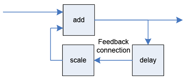
The feedback connection lies between the delay and the scaler modules, and redrawing the system to explicitly show the feedback yields the diagram below:
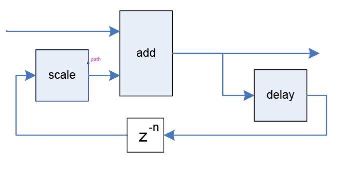
The total delay in the feedback path equals the blockSize+delay.currentDelay.
Portions of the MATLAB source file are shown below. Feedback connection is made with connect(SYS, 'delay', 'scale', 1); and feedback Pin Type is set with feedbackPinType.isComplex = -1;.
function SYS=feedback_delay_subsystem(NAME, MAXDELAY)

% ----------------------------------------------------------------------
% Set default input arguments
% ----------------------------------------------------------------------

if (nargin < 2)
    MAXDELAY=1024;
end

% ----------------------------------------------------------------------
% Creates the subsystem
% ----------------------------------------------------------------------

SYS=awe_subsystem('FeedbackDelaySubsystem', 'Recursive system implementing a feedback delay module');
SYS.name=NAME;

% Add the modules

add_module(SYS, adder_module('add', 2));
add_module(SYS, delay_module('delay', MAXDELAY));
add_module(SYS, scaler_module('scale'));

% Add input and output pins
pinType=new_pin_type;
add_pin(SYS, 'input', 'in', 'Audio Input', pinType);
add_pin(SYS, 'output', 'out', 'Audio output', pinType);

% Connect the modules together
connect(SYS, '', 'add.in1');
connect(SYS, 'add', '');
connect(SYS, 'add', 'delay');
connect(SYS, 'delay', 'scale', 1);

feedbackPinType.blockSize = -1;
feedbackPinType.numChannels = -1;
feedbackPinType.sampleRate = -1;
feedbackPinType.dataType = 'Inherit';
feedbackPinType.isComplex = -1;

SYS=set_feedback_pinType(SYS, SYS.connection{end}, feedbackPinType);

connect(SYS, 'scale', 'add.in2');


SYS.delay.currentDelay=MAXDELAY;
SYS.scale.gain=0.8;

% Add the GUI
add_control(SYS, '.scale.gain');
add_control(SYS, '.delay.currentDelay');

return;
Creating User Interfaces
Audio Weaver allows you to design custom user interfaces for audio modules and subsystems. The user interfaces are designed by MATLAB commands and translated into Audio Weaver script. The user interfaces created are drawn by the Audio Weaver Server and exist outside of the MATLAB environment. This section begins with a brief tutorial that demonstrates how to use existing user interfaces and to create interfaces for a custom subsystem.
Quick Tutorial
Run the example system agc_example.m. The script instantiates the system shown below and begins real-time execution.
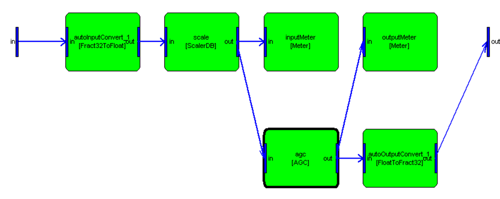
The script also draws the user interfaces, called inspectors, shown here:
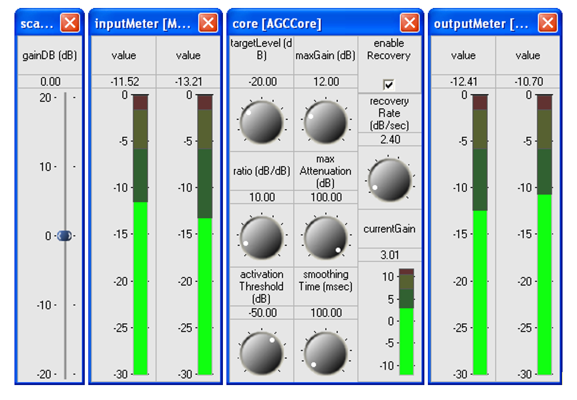
4 inspector panels drawn by the agc_example.m script.
Looking at the end of the agc_example.m file, the commands to configure the inspectors are:
SYS.scale.gainDB.range=[-20 20];
SYS.scale.gainDB.guiInfo.size=[1 3];
SYS.inputMeter.value.guiInfo.size=[1 3];
SYS.inputMeter.value.guiInfo.range=[-30 0];
SYS.outputMeter.value.guiInfo.size=[1 3];
SYS.outputMeter.value.guiInfo.range=[-30 0];
These commands specify the ranges of controls and their sizes on the inspector panels. The commands to draw the inspectors are:
awe_inspect('position', [0 0])
inspect(SYS.scale);
inspect(SYS.inputMeter);
inspect(SYS.agc.core);
inspect(SYS.outputMeter);
The first command, awe_inspect('position', [0 0]), specifies the screen position at which to draw the first inspector. The remaining 4 commands draw an inspector for each of the 4 internal modules. The inspectors are positioned from left to right (and the order of inspector drawing was purposefully chosen to mimic the audio signal flow in the subsystem.)
If you double-click on the title bar of a window, the inspector dialog may increase in size revealing additional "extended controls". For example, the scalerDB module reveals two more controls:
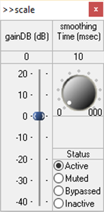
Double-clicking on the title bar returns the inspector to its "normal" size.
Using Controls
This section contains a few tips for using the inspector controls.
Clicking on a slider advances the control part way.
Grabbing and moving a slider updates the variable continuously.
An edit box directly above a slider or knob shows the current value. Clicking on an edit box allows you to type in a value.
Left clicking on a knob instantly turns the knob so that it is positioned over the click location.
Turn a knob by left clicking, and holding, a point on the knob. While you are actively turning a knob, you can increase the turn radius to more precisely adjust the value.
Knobs can wrap around from the minimum to the maximum value. Beware!
6.3. Creating Subsystem Control Panels
Now let us go a step further and draw a single control panel containing the individual inspectors for all 4 modules. Add the following lines prior to the "build" command within the agc_example.m script:
add_control(SYS, '.scale');
add_control(SYS, '.inputMeter');
add_control(SYS, '.agc.core');
add_control(SYS, '.outputMeter');
The first command exposes all of the controls from the internal module "scale" on the overall inspector. The second command exposes all of the controls from the "meter1" module and positions these controls to the right of the "scale" controls. This repeats for two more modules. The add_control.m commands add GUI information to the SYS object – they don't draw the controls themselves. After the system is built and running on the Server, the overall control panel is drawn by:
inspect(SYS)
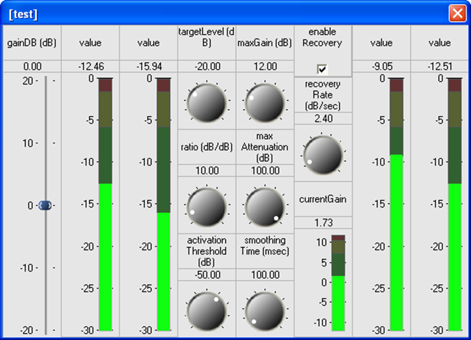
Overall inspector panel combining the individual controls from the 4 internal modules.
In this example, we combined several control panels into an overall control panel. The same process applies to adding controls for individual variables. The form of the command is similar, except that we specify the full path name of a variable as the second argument. For example, to expose only the "gainDB" and "targetLevel" variables, use the following commands:
add_control(SYS, '.scale.gainDB');
add_control(SYS, '.agc.core.targetLevel');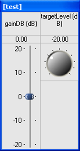
Ganging Controls Together
In certain applications, it is useful to have a single inspector control affect multiple variables on the target. For example, your audio system may have separate gains for left and right signals and instead of having two different inspector controls, you want a single control that affects both gain parameters. Tying a single control to multiple variables is referred to as ganging in Audio Weaver.
Consider the system shown in the figure below. This system is contained within the example script test_gui_ganged.m. The system has a stereo input, stereo output, and separate processing for the left and right channels. (Note that this is a contrived example since you could achieve the same result more easily and more efficiently by using stereo processing throughout.) To expose individual controls for the left and right gains, you would use the commands:
add_control(SYS, 'L.gain');
add_control(SYS, 'R.gain');
However, to gang the controls together, supply a cell array of variable names to the add_control command:
add_control(SYS, {'L.gain', 'R.gain'});
Both gain variables are then attached to the same inspector control.
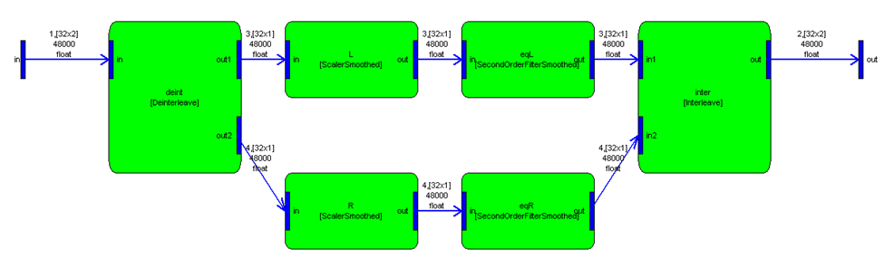
Example system used to demonstrate ganging of inspector controls.
Similarly, we can gang together the set of inspector controls for the second order filter modules. The second order filter module has six different controls; four are on the non-expanded panel and two are on the expanded panel:
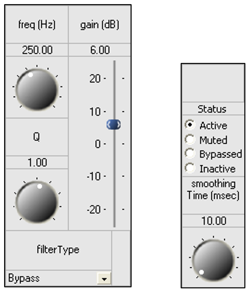
To gang together all inspector panels, use the commands:
add_control(SYS, {'eqL', 'eqR'}, 'right', 0);
add_control(SYS, {'eqL', 'eqR'}, 'right', 1);
The first command gangs together the controls for the base inspector while the second command affects the controls on the expanded panel.
There are a few things to keep in mind when ganging together controls. First, the same inspector value is written to all of the variables. If you need finer control, such as a balance control that uses different gains for different scalers, you'll need to develop a custom audio module with its own set function. Second, the variable updates are not truly simultaneous. Instead, they'll be separated by a few milliseconds in time. If you need truly simultaneous updates, then develop a custom inspector.
Overriding Default GUI Settings
Compare the combined inspector panel with the ones shown in the 4 inspector panels. All of the controls are there, but some of the (quite useful) labels shown in the window title bars are gone. For example, what do the first two level meters graphs correspond to? We can improve the combined inspector by overriding some of the variable names. By default, Audio Weaver utilizes the variable name as a label shown on the inspector. Override this default behavior by adding the command
SYS.meter1.value.guiInfo.label='Input Meter';
Prior to issuing the add_control(SYS, '.meter1') command. The inspector now draws as:
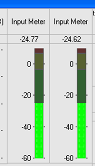
All of the default information needed to draw an inspector control comes from the detailed information within each awe_variable object. As we just saw, the default information can be overridden by setting fields within the variable's .guiInfo field. Other examples include:
Changing the range of a knob or meter:
SYS.agc.core.currentGain.guiInfo.range=[-5 5];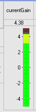
Note that the range information could have been changed in the awe_variable object itself:
SYS.agc.core.currentGain.range=[-5 5];
Changing it here would have restricted the range for both MATLAB usage and when drawing the inspector.Changing the units shown
SYS.agc.core.currentGain.guiInfo.units='dB';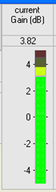
As before, the units information could also have been incorporated into the awe_variable object itself (which would have been a better idea!)
Changing Control Sizes
Audio Weaver uses a set of normalized coordinates when drawing controls. The coordinates are chosen such that a knob has a size of exactly 1 X-unit by 1 Y-unit:
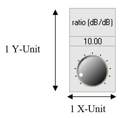
Sliders and meters each have a size of 1 X-unit and 2 Y-units:
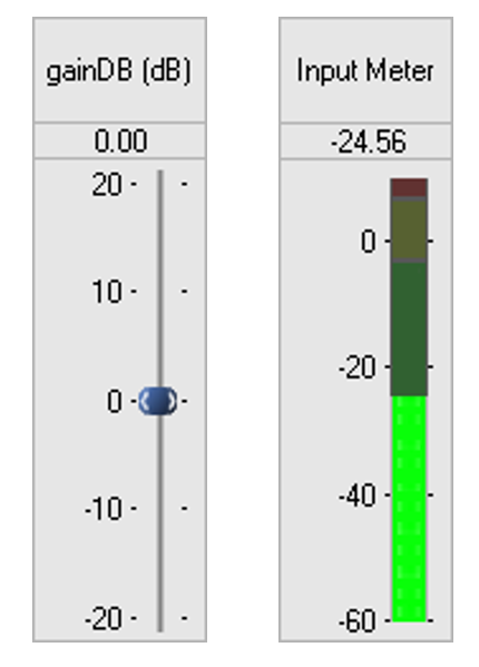
By setting the control sizes to be simple multiples of an underlying normalized coordinate system, it is easy to position multiple controls in groups:
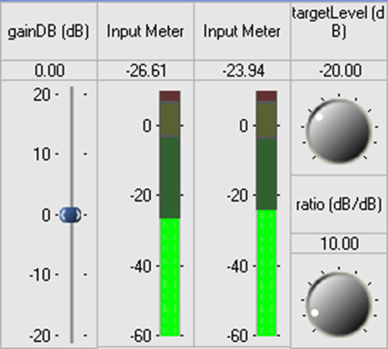
You can also override the default size of a control by modifying the .guiInfo field. For example, the knobs and sliders in the overall dialog shown in the combined inspector panel have been vertically aligned by setting the control sizes:
SYS.scale.gainDB.guiInfo.size=[1 3];
SYS.inputMeter.value.guiInfo.size=[1 3];
SYS.outputMeter.value.guiInfo.size=[1 3];
Changing the Inspector Layout
The inspector panel shown in the combined inspector panel consists of 4 separate "sub-inspectors", one for each internal module. By default, Audio Weaver draws sub-inspectors and individual controls from left to right. Subsequent controls are added to the right of the last control.
An optional 3rd argument to add_control.m allows you to specify the position of the control. The syntax is:
M=add_control(M, HNAME, POSITION)
where POSITION is either:
A 1x2 vector [offsetX offsetY] of normalized control units. The control is drawn at position [X Y] + [offsetX offsetY] where [X Y] is the position of the last control drawn.
One of the relative positioning strings 'right', 'topRight', 'below', 'bottomLeft', or 'bottomRight'. The control is drawn relative to the position of the last control. This is described below.
The difficulty with using the [offsetX offsetY] syntax is that you must know the size of the last control drawn in order to effectively use this form of the command. The relative positioning strings are much more useful and we focus on their usage below.
The 'right' command positions the next control immediately to the right of the last control added. The 'below' command positions the next control immediately below the last control added. The 'topRight' command positions the next control at the top edge of the dialog to the right of the right-most control. The 'bottomLeft' command positions the next control at the bottom edge of the lowest control all the way to the left. The 'bottomRight' command positions the next control below the lowest control and to the right of the right most control. A few examples will make this clear.
Consider the group of controls shown below:
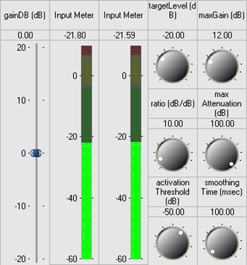
"gainDB" is the first control drawn and always appears at the top left corner of the inspector dialog.
"Input Meter" is drawn to the "right" or "topright" of "gainDB".
"targetLevel" is drawn to the "right" or "topright" of "InputMeter".
"ratio" is drawn "below" "targetLevel"
"activationThreshold" is drawn "below" "ratio".
"maxGain" is drawn to the "topright" of "activationThreshold".
"maxAttenuation" is drawn "below" "maxGain".
"smoothingTime" is drawn "below" "maxAttenuation".
Another way to understand the relative positioning strings is to consider the controls being drawn in a matrix:
"right" positions the next control one column to the right of the last control.
"below" positions the next control one row down from the last control.
"topRight" starts adds a new column to the right edge and positions the next control in the first row.
"bottomLeft" adds a new row at the bottom and positions the next control in the first column.
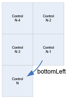
"bottomRight" adds a new row at the bottom and and to the right.
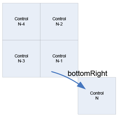
Inspector Control Types
We have so far seen several different types of controls: knobs, sliders, meters, and checkboxes. There are several other types of controls and the default control type is assigned based on the following logic. The following steps are evaluated from start to finish and terminate when a suitable match is found.
If the variable is an array, then controlType='grid' and the following is drawn:
If the variable has usage 'const', then controlType='const' and the variable is drawn as a read-only edit box
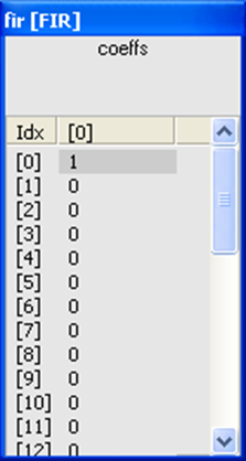
If the variable has no range information, then controlType='edit' and it is drawn as an edit box:
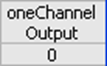
If the variable has usage 'parameter', has type 'int', and there are only two items, then controlType='checkBox'
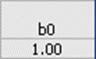
If the variable has usage 'parameter', has type 'int', and there are three to nine items, then controlType='dropList'. For each allowable integer value, you can specify a string to provide an easy-to-read drop list.
If the variable has usage 'parameter', has type 'int', and there are 10 or more items, then controlType='knob'. Or, if the variable has usage 'parameter' and type 'float', then controlType='knob'.

If the variable has usage 'state', has type 'int' and has exactly two items, then controlType='LED'.
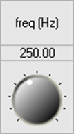
If the variable has usage 'state', has type 'int' and has three or more items, then controlType='meter'. Or, if the variable has usage 'state' and type 'float', controlType='meter'.

Otherwise, a default controlType cannot be assigned to this variable.
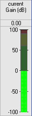
The default .controlType string can be overridden. For example, the agc_core_module.m uses a knob for the recoveryRate control. You can change this to a slider using the command:
SYS.agc.core.recoveryRate.guiInfo.controlType='slider';
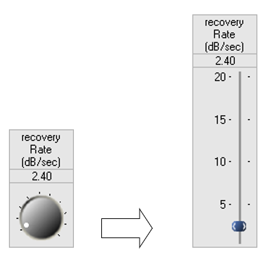
Module Status Control
An audio module can be in one of four run-time states: Active, Muted, Bypassed, and Inactive, as described in Real-Time Tuning. The module status is set using a group of radio buttons. To add a module status control, use the syntax:
add_control(SYS, '.moduleName.moduleStatus');
where "moduleName" is the name of the module. The control has a normalized size of 1 by 1 and appears as shown below:
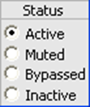
Note that the variable "moduleStatus" does not exist within the module. Instead, special case code is used to instantiate this control.
Drawing Arrays of Controls
The default controlType assigned to an array variable is a grid control. The grid control displays a 2-dimensional matrix of values and is similar to an Excel spreadsheet. There are times when an array of controls (knobs, sliders, meters, etc.) is more convenient than a grid control. For example, consider a 4-input 2-output mixer_module.m The mixer gains are stored in a 4 x 2 matrix .gain of cofficients and the default inspector interface would appear as:
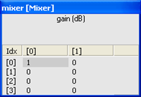
Mixers are typically drawn with knobs. Would it be possible to draw an "array of knobs"? Yes, simply override the controlType by setting
SYS.mixer.gain.guiInfo.controlType='knobs';
The inspector then draws as:
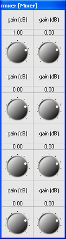
This is getting closer, but not exactly what is wanted. Mixer interfaces typically have each column dedicated to an input channel and each row dedicated to each output. We need to transpose the array of coefficients:
SYS.mixer.gain.guiInfo.transposeArray=1;
This yields the final mixer interface, which is in fact specified in the mixer_module.m script.
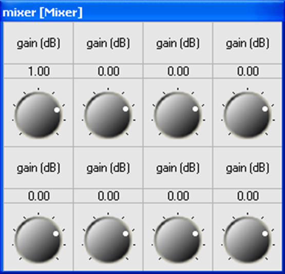
Certain other modules use arrays of controls when drawing themselves. For example, the meter_module.m is designed to operate on multichannel signals and uses a separate meter control for each audio channel. The meter_module.m script overrides the default grid control with a 'meter' module. The interfaces shown in 4 inspector panels and the Overall inspector panel have two controls shown for both the meter1 and meter2 modules. That is because these modules are displaying stereo information and thus a pair of meters is shown.
Base and Extended Controls
We saw in the Quick Tutorial that some inspectors could toggle between showing and hiding an "extended" panel by double-clicking on the title bar. (Note that this only works for inspectors drawn by the Server; not by inspectors drawn by the Designer GUI.) Typically, the frequently used controls appear on the base panel while the less frequently used items, such as the module status, appear on the extended panel.
Controls are placed on the extended panel via an optional fourth argument to the add_control.m command. The full syntax of the command is:
M=add_control(M, HNAME, POSITION, ISEXPANDED)
ISEXPANDED is a Boolean, and if it equals 1, the control is placed on the extended panel. By default, ISEXPANDED=0 which places the control on the normal panel. When creating an inspector for a module, you should first add all of the controls that appear on the normal panel and then add all of the controls that appear on the extended panel. Extended controls can appear to the right of, or below, the standard controls.
The interpretation of ISEXPANDED is also slightly different when adding a set of controls from an internal module to a high-level inspector. In this case,
ISEXPANDED=0 – Add all of the controls from the base panel of the internal module to the base panel of the overall inspector.
ISEXPANDED=1 – Add all of the controls from the extended panel of the internal module to the extended panel of the overall inspector.
ISEXPANDED=2 – All of the controls – including the extended ones – appear on the normal control panel.
In some cases, you call add_control.m twice for the same module to position controls on both the base and extended panels:
add_control(SYS, '.agc.core', 'topRight', 0);
add_control(SYS, '.agc.core', 'topRight', 1);
Further Control Attributes
An "attribute string" specifies additional details regarding how a control is drawn. The attribute string provides fine grained control over, for example, the number of tick marks displayed or the numeric values at which tick marks are displayed. The attribute string information is control-specific and consists of a set of key/value pairs: "key1=value1 key2=value3". Note that there is a space between key value pairs and not a comma. The attribute string is contained within the .guiInfo.attribStr field.
The list of attributes is fairly lengthy. A few commonly used attributes are called out below.
Logarithmic knob or slider. In audio, it is useful to have a knob that acts on a logarithmic scale for controlling frequency. To enable this, set:
module.variable.guiInfo.attribStr='mapping=log';
You can see an example of this within the sine_gen_module.mRestricting knobs and sliders to even values:
module.variable.guiInfo.attribStr='stepSize=2';Converting a linear value to dB for meter display. Often an audio module performs calculations in linear space whereas the preferred display is in dB. Instead of performing the linear to dB conversion on the target, you can perform it in the meter itself. Use:
module.variable.guiInfo.attribStr='mapping=db20';
Grid Control Attributes
format=format_specifier – a printf style format to use when formatting values, default %g
min=val – default –1e10, the minimum displayable value on the grid
max=val – default 1e10, the maximum displayable value on the grid
colwidth – default 50, value must be >= 50, width of column in pixels
sidewidth – default 30, value must be >= 30, width of first column in pixels
Edit and Constant Control Attributes
format=format_specifier – a printf style format to use when formatting values, default %.2f
stepsize=step – default 0, the amount by which displayed values will be quantized
min=val – default -100, the minimum displayable value on the meter
max=val – default 0, the maximum displayable value on the meter
readonly – 0 or 1, default 0; when set prevents the user editing the value
Checkbox Control Attributes
readonly=val – 0 or 1, default 0; when set prevents the user changing the selection
Drop List Control Attributes
readonly=val – 0 or 1, default 0; when set prevents the user changing the selection
Knob and Slider Control Attributes
min=val – default 0, the minimum value of the slider
max=val – default 1, the maximum value of the slider
value=val – default 0, the initial position of the slider
format=format_specifier – a printf style format to use when formatting values, default %.2f
units=units_name – no default, used to name the units, for example dB
mapping=[log|lin[ear]] – default linear. The value is displayed according to the mapping. Log is not possible unless min > 0.
ticks=nTicks – default is 2, range is 2-32, this is the number of tick marks to display
useticks=[0|1] – default is 0, when 1, tickmarks are drawn
fixedticks=nFixedTicks – default is 2, range is 2-32, this is the number of fixed ticks to display
tickmarks=v1, … , vN – a list of labels to apply to tickmarks up to a maximum of 8 values, no default
stepsize=step – default 0, the amount by which displayed values will be quantized
control=[knob|slider] – default slider. If knob, a rotary knob control is shown instead of a slider.
height=val – default is natural control height, values larger than default stretch the control vertically downwards. If control=knob, this value is ignored. Do not set this value. The height is automatically calculated based on guiInfo.size.
continuous=[0|1] – default 1, when 1, all changes are assigned as they happen, otherwise changes are sent only when the user releases the mouse
muteonmin=[0|1] – default 0, when 1, the underlying variable is set to 0 when the slider/knob is turned to its minimum value. This is useful for dB controls which should mute when turned all the way down.
LED Control Attributes
There are no attributes associated with the LED control.
Meter Control Attributes
format=format_specifier – a printf style format to use when formatting values, default %.2f
units=units_name – no default, used to name the units, for example dB
mapping=[db20|undb20|lin[ear]] – default db20. The value is displayed according to the mapping.
ticks=nTicks – default is 2, range is 2-32, this is the number of tick marks to display
useticks=[0|1] – default is 0, when ,1 tickmarks are drawn
tickmarks=”v1, … , vN” – a list of labels to apply to tickmarks up to a maximum of 8 values, no default
stepsize=step – default 0, the amount by which displayed values will be quantized
meteroffset=offs – default 0, an amount to be added to values before use
min=val – default -100, the minimum displayable value on the meter
max=val – default 0, the maximum displayable value on the meter
height=val – default is natural control height, values larger than default stretch the control vertically downwards. Do not set this value. The height is automatically calculated based on guiInfo.size.
Module Level .guiInfo
We've seen how a variable's .guiInfo field can be used to customize the control attached to it. Modules and subsystems also have a .guiInfo field that can be used to modify the appearance of their inspector panel. Two characteristics of the inspector panel can be customized:
M.guiInfo.showMore – a Boolean value that specifies whether the normal inspector (=0) or the extended inspector (=1) should be initially shown. By default, showMore=0 and the normal inspector appears.
M.guiInfo.caption – specifies the string that should appear in the inspector's title bar. By default, this is empty and the dialog title bar contains the string:
moduleName [className]
Flash File System
Some hardware targets provide on-board flash memory configured to work with Audio Weaver. The flash memory stores files, usually compiled Audio Weaver Scripts, that execute upon boot up. This feature allows the hardware target to operate in standalone mode, that is, without having a PC attached.
When the Server connects to a hardware target, the target reports back its capabilities and features to the Server. This information is displayed within the Server's Output Window. One of the lines shown indicates whether the target provides a Flash File System:
Is FLASH supported: Yes
Accessing the Flash File System Using MATLAB
This section describes how to access the Flash File System using MATLAB commands.
Flash Memory Directory
To obtain a directory of files residing in flash memory, use the command
target_flash_dir
This prints the directory information in the MATLAB output window. To get directory information programmatically, use
L=target_flash_dir;
The function returns an array of structures, one per file, with the following fields:
.fileName – name of the file (string)
.attrib – attribute byte described as below.
The attribute byte is also dissected into separate Boolean fields for ease of use:
.isStartup
.isCompiled
.isAWS
.isPreset
Adding Files
Files are added one at a time using the command
target_flash_add(FILENAME, ATTRIB)
where FILENAME is a string specifying the file to add along with absolute or relative file path and ATTRIB is the 8-bit attribute byte discussed as below.
Attribute Byte | Description |
|---|---|
24 | Compiled Script file (non-bootable) |
26 | Compiled Script file (bootable) |
40 | Compiled Preset File (non-bootable) |
42 | Compiled Preset File (bootable) |
FILENAME must be at most 24 characters in length, for example “agc_example.awb”; this is checked by the function. The function also checks that FILENAME does not already exist in the Flash File System.
Deleting Files
To delete individual files use
target_flash_delete(FILENAME)
where FILENAME is the name of the file to delete. To completely erase flash memory – essentially reformatting it – use
target_flash_erase
This command takes several seconds to execute. The command executes without prompting you to confirm the erasure.
Creating and Compiling Files
The MATLAB command awe_diary.m is the primary method for creating Audio Weaver Script (.aws) files. This command is discussed in awe_diary.m and essentially captures all of the commands sent from MATLAB to the Server and logs them to a specified file. Typically, you wrap the building of a system in pairs of awe_diary commands as shown below:
awe_diary('on', 'myscript.aws');
build(SYS);
test_start_audio;
awe_diary('off');
In this example, all of the commands needed to build the system SYS on the target are captured in the file myscript.aws.
The next step is to convert the Audio Weaver Script file (.aws) in a binary file (.awb). The command to use is
awe_compile(AWSFILE, AWBFILE, RELATIVE, MAXMESSAGELENGTH);
where
AWSFILE – input Audio Weaver Script file name.
AWBFILE – output compiled script file name.
RELATIVE – specifies whether the generated .awb file should use relative addressing. This is a deprecated feature and must always be set to 1.
MAXMESSAGELENGTH – maximum message length in the generated .awb file, in words. When building a system and you are connected to an embedded target then the message buffer size of the embedded target is used and this argument is ignored. Only use when you are generating the .awb file on the PC and want to limit the message buffer size. MAXMESSAGESIZE must be in the range of 16 to 264.
Flash Manager Example
This section concludes with an example of how to utilize the flash memory manager in practice. We store one of the Audio Weaver example systems in flash and configure the board to execute the script upon boot up. Both compiled and text commands are stored. The compiled files are executed when the DSP boots; the text script files are executed when the Server connects. We will use the automatic gain control system and build the system and create a preset using MATLAB.
Startup Audio Weaver using the awe_init.m command.
Then create the automatic gain control example system. Use the diary function to capture all of the Server commands:
CODEawe_diary('on', 'agc_example.aws'); SYS=agc_example; awe_diary('off');The system is returned in the variable SYS.
Execute the agc_example.aws file in AWE Server from File->Execute Script…. This will run AGC example on the target and the user interface is also drawn.
Using the inspectors, tune the system to an audibly different state. In this example, lowering the targetGain variable of the AGC Core to -40 dB will make the audio much quieter.
Using the Flash Memory Manager, compile the script
agc_example.aws → agc_example.awbNow store the compiled script file in the flash file system and mark it as shown:
agc_example.awb Compiled Script. Boot file. Attrib=26
Ensure that there is only one file in the flash file system.Shut down the Audio Weaver Server and reset the target. The target will execute agc_example.awb at boot time and you'll immediately hear audio being processed.
Manually launch the Server. The Server will connect and it shows CPU usage and memory usage of the agc_example.awb running on the target.