
Visualization of Signals in AudioWeaver
About This Application Note
The Visualization of Signals in AudioWeaver Application Note describes the various methods that can be used to visualize a signal in AudioWeaver.
Sink Display Module
The Sink Display module copies data at the input pin and stores it in an internal buffer. The module can be found in Sinks->Sink Display in the Module Bar on the left-hand side of AudioWeaver Designer.
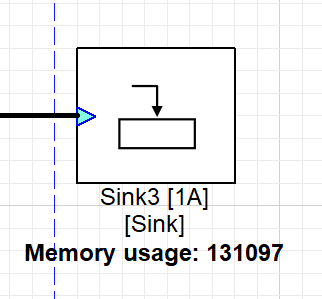
Figure 1: Sink Display Module
There are four variants of this module: -
Sink Display: Copies data at the input pin and stores it in an internal buffer.
Sink Display with Properties: In addition to the normal Sink Display functions, this module makes the wire information available as internal variables. Block size, channel number, sample rate and signal complexity can be accessed in MATLAB code, source code, or in a layout using the ParamGet module.
Sink Display Fract32: The module captures a block of fract32 input data and stores it into an internal buffer.
Sink Display Fract32 with Properties: Similar to Sink Display with Properties module.
Sink Display Int32: The module captures a block of integer input data and stores it into an internal buffer.
Sink Display Int32 with Properties: Similar to Sink Display with Properties module
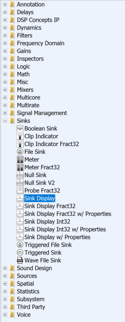
Figure 2: Location of Sink Display Module
Overall Control
The Sink Display gives multiple methods by which the user can control the plotting of the input data, which is known as ‘Overall Control’. In Overall Control the user can choose between Time Domain, Frequency Domain, Index and Custom.
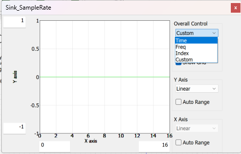
Figure 3: Sink Display Overall Control
Time Domain: A time-domain graph displays the changes in a signal over a span of time. In the figure below we are inputting a Sine Tone at 1KHz with 48000Hz Sample Rate with a Block Size of 768 into the AudioWeaver Designer. This translates to ~16 sine cycles (peaks and troughs) in our time window which is ~16 msec as seen below in Fig. 4.
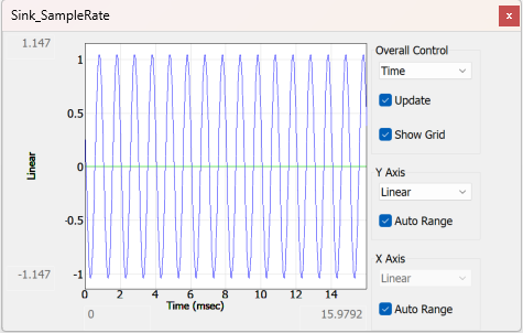
Figure 4: Sink Display Time Domain
Frequency Domain: Frequency domain displays how much of the signal exists within a given frequency band concerning a range of frequencies. We are using the same example of inputting a Sine Tone at 1KHz with 48000Hz Sample Rate into the AudioWeaver Designer. In Fig.5 we can see that in this domain a signal of amplitude of ~0.4 peaks at 1KHz in Hz.
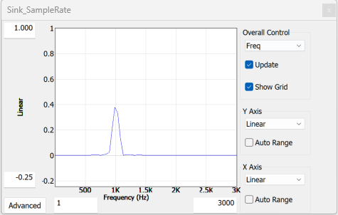
Figure 5: Sink Display Frequency Domain
Meter Module
The Meter module provides a flexible level meter that can operate in several modules. The module has a single multichannel input and separate meters for each channel. The meter can be configured to conform to IEC 60280-10 (peak meters) and IEC 60280-17 (VU Meter) specifications.
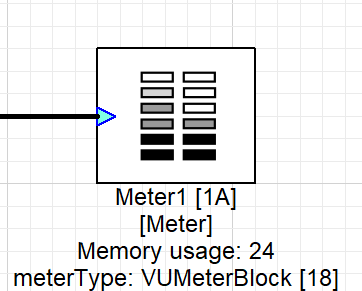
Figure 6: Meter Module
There are two variants of the module: Meter and Meter Fract32 modules. The Meter modules can be found in Sinks->Meter in the Module Bar on the left-hand side of AudioWeaver Designer.
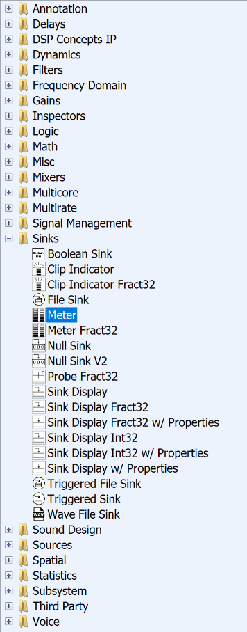
Figure 7: Meter Module Location
Variables
Right click on the module, go to properties, and switch tabs to get to variables. Operation modes of the meter selects between Peak and RMS calculations under variable ‘meterType’.
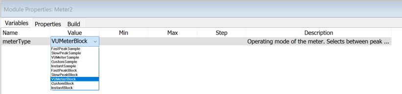
Figure 8: Meter: Variables
The following are the modes:
In meterTypes 0 to 4, the peak attack and release are performed on a sample-by-sample basis in the envelope follower. In meterTypes 16 to 20, the peak absolute value for the entire input block is found and this one value is passed through the envelope follower.
Value | Arguments | Description |
0 | FastPeakSample | The meter implements a peak meter according to IEC 60280-10 in "fast mode". The attackTime is fixed at 5 msec and the release time is fixed to 1087 msec. |
1. | SlowPeakSample | The meter implements a peak meter according to IEC 60280-10 in "slow mode". The attackTime is fixed at 10 msec and the release time is fixed to 1450 msec. |
2. | VUMeterSample | The meter implements a meter according to IEC 60280-17. This corresponds to the industry standard "VU meter" definition. The attack and release times are 65 msec. |
3. | CustomSample | The meter implements a custom peak meter. You have to manually set the attackTime and releaseTime from a MATLAB script. |
4. | InstantSample | The meter is instantaneous and has attack and release times of 0 msec. The meter value equals the last value in each block. |
16. | FastPeakBlock | The meter implements a computationally cheap approximation to IEC 60280-10 in "fast mode". The attackTime is fixed at 5 msec and the release time is fixed to 1087 msec. |
17. | SlowPeakBlock | In SlowPeakBlock mode the attackTime is fixed at 10 msec and the release time is fixed to 1450 msec. |
18. | VUMeterBlock | The attack and release times are 65 msec. |
19. | CustomBlock | Same as CustomSample mode. |
20. | InstantBlock | Same as InstantSample mode. |
Rebuffer Module
The Rebuffer module is a Multirate module. The module overlaps data into larger block sizes while keeping the underlying time base preserved. The module can be found in Multirate->Rebuffer in the Module Bar on the left-hand side of the AudioWeaver Designer.
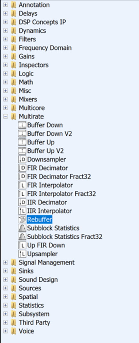
Figure 9: Rebuffer Module Location
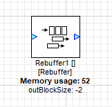
Figure 10: Rebuffer Module
Module Functional Description
A Rebuffer module converts from a smaller to a larger block size, with overlap. The module can support an arbitrary number of channels and supports any 32-bit data type (integer and floating-point). An internal buffer holds the overlap between samples.
At instantiation time, the output block size is specified by the variable OUTBLOCKSIZE. If OUTBLOCKSIZE is positive (e.g., 64), then a specific output block size (64) is set. If OUTBLOCKSIZE is negative (e.g., -2), then this specifies that the output block size is 2 times that of the input block size.
Note that the rate of output blocks equals the rate of the input blocks. That is, this module does not change the fundamental block time.
Arguments
Arguments can be found Rt Click -> View Properties -> first tab in the properties as shown.
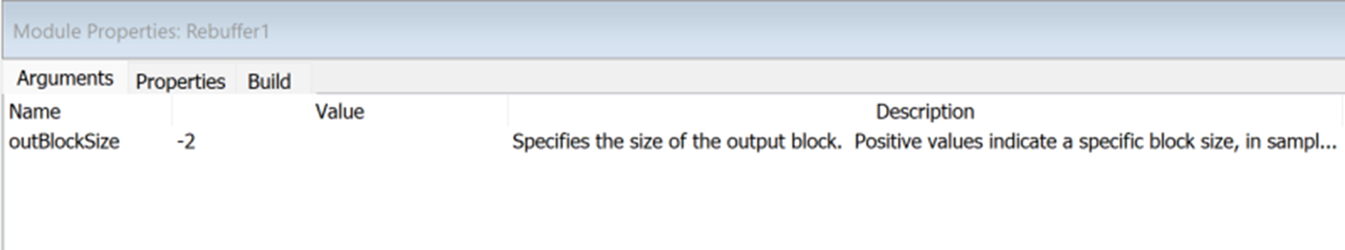
Figure 11: Argument Tab for Buffer Module
Arguments | Description | Default Value | Range |
outBlockSize | Specifies the size of the output block. Positive values indicate a specific block size, in samples. Negative values specify a multiplicative factor between the input and output block sizes. | By default, outBlockSize = -2. | -32:100000 |
Signal Visualization Examples
Input Signal to Meter and SPL Sink Display
In this example we will be using an input signal of 1kHz Sine Tone via two input channels. The Meter module is selected in VUMeterSample mode and represents the amplitude of the input signal. In this example we are converting the input signal into an SPL output of dBA weighting by inputting the microphone sensitivity in the ScaleOffset module as shown below with the arrow. The SPL_Display sink plots a graph of the SPL level of the input channels (in dBA) as shown in the purple blocks. You can also verify the sample rate of the input signal by using the sink display again and counting the number sine cycles present in the window as shown in the green box highlights. The Sample Rate is calculated by
Sample Rate = (Block Size / No of cycles in window) * Sine Tone Freq
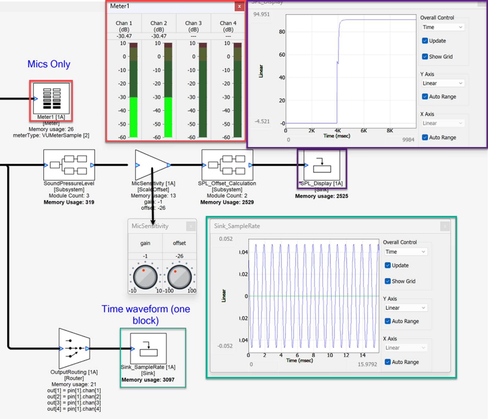
Figure 12: SPL Display and Meter Example
Rebuffer to Sink Display
One of the many use cases of a Rebuffer module is that it can be used to visualize a signal. In the example below, the two consecutive signals cannot be completely visualized by the inherent wire properties which is 2x256. i.e., 2 channels with block size as seen in Sink2. After applying a Rebuffer module of outBlockSize = -256, which means that Output = 256 x Input Block Size which comes out to be 65536 in the example. We can visualize both the wave interactions within the Sink3 SinkDisplay window. In this example the Bell tone is being played by two Wave One Shot Players at a particular order. In Sink2 it is difficult to figure out the order of the wav files being played whereas Sink3 with the rebuffer makes the order of the wav files clear.
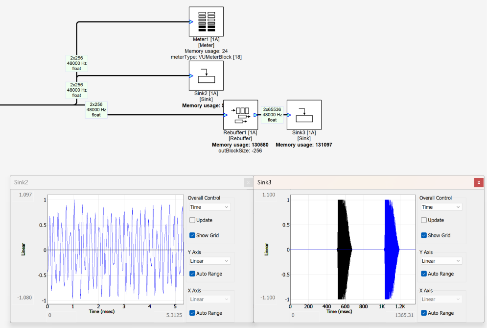
Figure 13: Rebuffer to Sink Display
Block Statistics to Rebuffer
The Block Statistics module calculates statistics of the input signal on a block-by-block basis. The input pin can have an arbitrary number of interleaved channels and the calculation occurs over all channels. The output pin has a single channel and a blockSize of 1.
The variable for BlockStatistics module is statisticsType which specifies which statistic is computed: 0=maximum, 1=minimum, 2=maximum absolute value, 3=mean, 4=RMS, 5=standard deviation, 6=variance, 7=average energy, 8=sum, 9=sum of squares. The statistics are computed on a block-by-block basis and stored in the instantaneousValue variable.
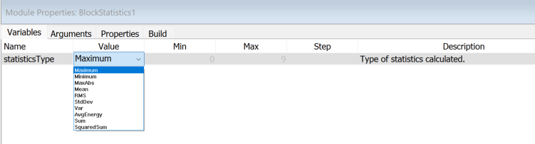
Figure 14: Block Statistics: Arguments Tab
The example below we are checking the input signals for Discontinuities. The Block Statistics module outputs the maximum difference between the reference signal in this case which is 800Hz sine tone and input signal block by block and outputs the value. By just adding the sink display we are unable discern between the change of signal. By adding a rebuffer module we can visualize as well as correlate the exact location of the discontinuities in real time. The green highlight in the graph corresponds to the first discontinuity as seen in the window below, whereas the orange highlight is for the second discontinuity.
We can minimize the post analysis and debugging of a signal significantly by visualizing it in real time in AudioWeaver.
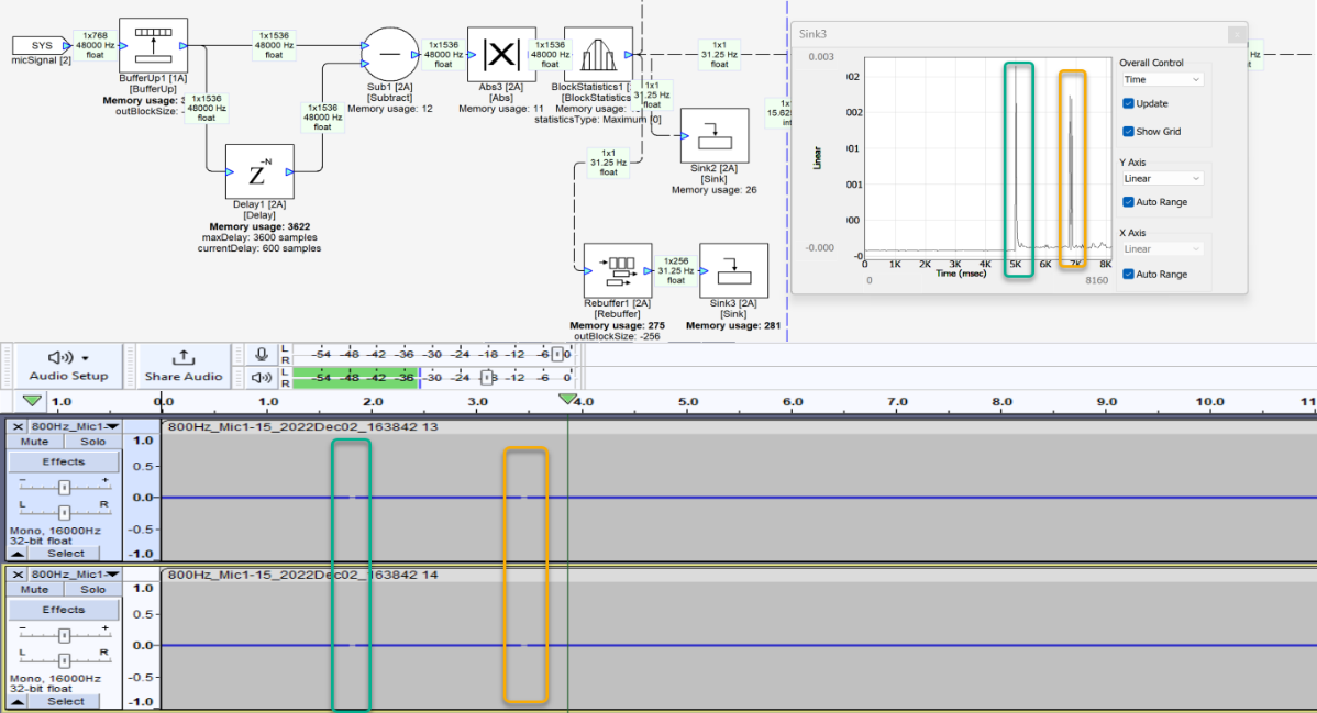
Figure 15: Block Statistics to Rebuffer example