
Multirate
This section contains the following pages:
General Information
Audio Weaver is able to process signals at different sampling rates all within the same layout. This was seen with control signals but the feature is much more powerful. Audio Weaver is able to handle multirate processing in two different ways:
Single block time processing
Multiple block time processing
In single block time processing all of the audio modules execute within a single thread at the same rate. In multiple block time processing there are multiple threads on the target processors and different block times execute within separate interrupt levels. Each approach is described in turn.
Single Block Time Processing
A module has an associated block size and sampling rate. We’ve been treating these wire properties as separate information but when combined they yield the block time, also referred to as block rate, of a module. For example, consider the system shown below.
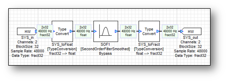
The sampling rate is 48 kHz and the block size is 32 samples. Each block of audio thus represents 32 / 48000 = 2/3 msec of audio. 32 sample audio buffers arrive every 2/3 msec and each block executes in turn.
There are a number of modules which can be used to change the sampling rate and still maintain the same block time. 4 Examples are listed below:
 | Upsampler | Inserts zeros between samples. No filtering |
 | Downsampler | Discards samples. No filtering. |
 | FIRInterpolator | Upsampler followed by an FIR interpolating filter. Filter coefficients are calculated automatically |
 | FIRDecimator | FIR filter followed by a Downsampler. Filter coefficients are calculated automatically |
Additionally, see the IIR Interpolator, IIR Decimator, and the Up FIR Down modules for further examples of modules that can change the sampling rate of the system without changing the block rate.
The Upsampler and Downsampler modules insert zeros and discard samples, respectively. Specify the up and downsampling factors on the Arguments tab of the Module Properties page. The downsampling factor must be chosen so that it divides the input block size and yields an integer number of output samples. Consider the system shown below:
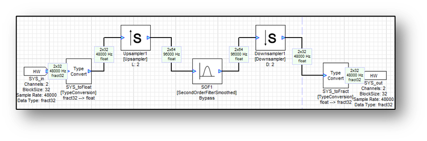
As before, the input block time is 2/3 of a millisecond. The Upsampler module is configured for an upsampling factor of L=2. The output sampling rate is 96 kHz and the block size is now 64 samples. Note that 64/96000 = 2/3 millisecond and the block time is preserved. As before, all modules execute every 2/3 millisecond.
The Upsampler and Downsampler modules correspond to standard up and downsamplers found in DSP text books. Since they lack any filtering, they are rarely used.
The FIRInterpolator and FIRDownsampler modules, on the other hand, contain FIR filters. The FIRInterpolator inserts zeros and then filters the resulting signal with a lowpass filter; the FIRDecimator first applies an FIR lowpass filter and then decimates. Both modules use an efficient polyphase implementation to reduce the processing load. These modules also preserve the underlying block time.
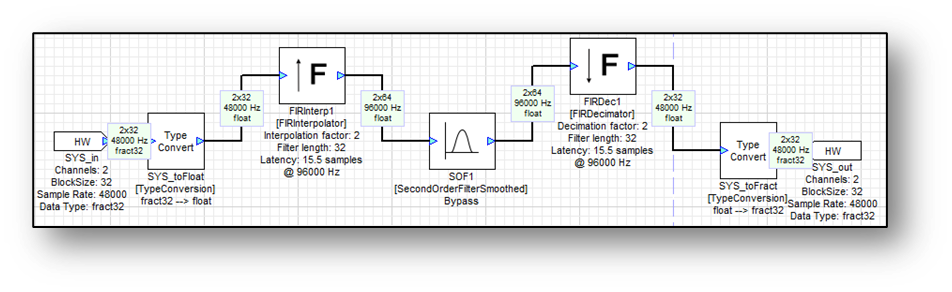
On the module properties for the FIRInterpolator / FIRDecimator specify the up / downsampling factor as well as the length of the FIR filter. The length of the FIR filter must be an integer multiple of the up / downsampling factors. When the modules are instantiated the FIR filter coefficients are computed using a Hamming window. Advanced users can change the filter coefficients by using MATLAB scripts.
The Rebuffer module stores and overlaps buffer data into larger block sizes, allowing for more data to be displayed.
 | Rebuffer | Overlaps input data into larger output blocks, allowing for longer time displays. |
The Rebuffer can accept data of any type. In its module properties is a variable called “outBlockSize,” which allows the user to set the output block size for the module. If a positive value is entered, that value is used as the output block size. If a negative value is entered, the value is used as a multiplier to the input block size. For example, an outBlockSize of 32 will yield an output of block size 32, and an outBlockSize of -8 yields an output with 8 times the block size of the input.
For example, the following block diagram shows a SinSmoothedGen source wired directly to a Sink module, which can be used to plot the input data:
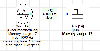
However, the Sink display shows only a small amount of data (in this case, 0.67 msec, based on the example above with a block size of 32 and sample rate of 48000 Hz):
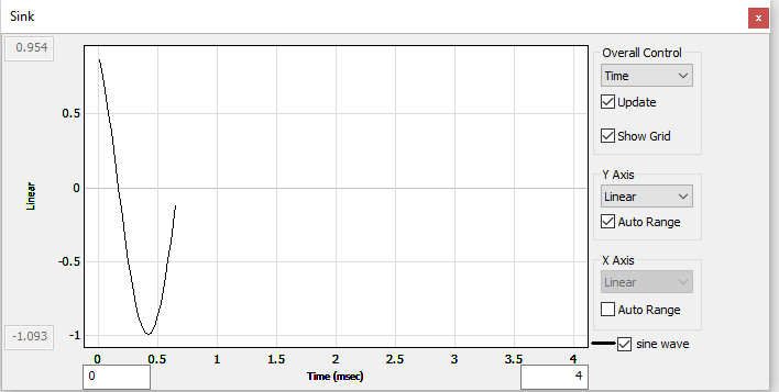
4 ms Sink display showing 32 samples of a sine wave
To extend the amount of displayed data, a Rebuffer module with outBlockSize -8 is added between the SineSmoothedGen and Sink modules:
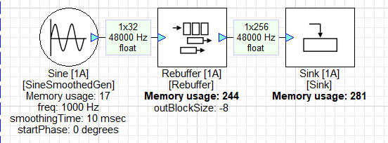
Note that the input block size to the Sink module is now 256 - a factor of 8 from the initial 32 sample block size. The Rebuffer now allows the Sink module to display 8 times the amount of data, easily spanning the 4-msec window:
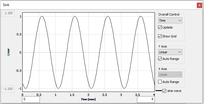
4 ms Sink display showing samples of a sine wave after Rebuffer module with output of 256 samples
The Rebuffer module is also useful for multirate processing. The Rebuffer module increases the output block size while keeping the sampling rate and block time constant. It achieves this by outputting blocks which overlap in time. Consider the system shown below. The input block size is 32 samples and the Rebuffer module is configured to output 128 sample blocks.
Each block that is output overlaps the previous one by 96 samples as shown below.
Overlapping data in output blocks from a Rebuffer module
The Rebuffer module is useful for frequency domain processing when it is necessary to have a certain amount of overlap between blocks. The inverse of the Rebuffer module is the BlockExtract module. This module extracts a subset of samples and reduces the block size.
Multiple Block Time Processing
In some applications processing needs to be performed at multiple block times. Consider a system that has low latency processing with a block size of 32 samples combined with frequency domain processing at a block size of 256 samples. At a 48 kHz sampling rate, the 32 sample processing would occur every 2/3 millisecond while the 256 sample processing would occur every 5 1/3 millisecond. In Audio Weaver, this ratio of block rates is called the clockDivider. In the example above, the clockDivider would be 1 for the 32 sample processing, and 8 for the 256 sample processing.
Note: even though it’s a single AWD layout that can have multiple clockDividers, behind the scenes there is a distinct sublayout created for all the processing for each unique clockDivider.
Multirate processing can be achieved using the BufferUp and BufferDown modules to manipulate the clockDividers of the signal processing layout.
 | BufferUp | Buffers up to larger blocks without overlapping, clockDivider is set to ratio of output block size and input block size. |
 | BufferUpV2 | Same as Buffer Up module, but can also modify LayoutSubId to control which thread a layout runs on. |
 | BufferDown | Buffers down to smaller blocks without dropping samples. |
 | BufferDownV2 | Same as Buffer Down module, but can also modify LayoutSubId to control which thread a layout runs on. |
The BufferUp module generates larger non-overlapping blocks. On the module properties dialog specify the output block size either as an integer number of samples or as a multiple of the input block size by using a negative number. In the example above, to go from 32 to 256 samples, specify a 256 sample block size (or a multiplier by specifying -8). To return to a 32 sample block size, use the BufferDown module. Again, explicitly specify the output block size either as an integer number of samples or as a divider.
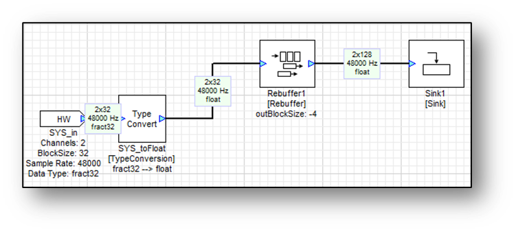
The system shown below combines 32 and 256 sample block sizes.
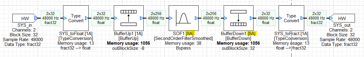
Simple multirate example system
The highlighted portion of the figure above shows the label ‘[8A]’ for the SOF1 and BufferDown1 modules. This annotation indicates that these modules execute in a separate sublayout at a rate of 1/8th (clockDivider of 8) compared to the primary layout.
Note: the ‘A' in the annotations means that the LayoutSubId (or threadId) is 'A’ for this sublayout. The LayoutSubId can only be changed by the Buffer Up/Down V2 modules. More on this in the Multithread Processing below.
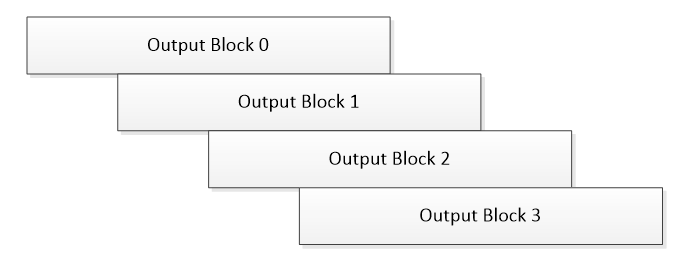
The output of the BufferUp1 module contains 256 samples which equals 8 32-sample blocks. The output is non-overlapping as shown here.
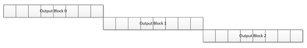
Non-overlapping output blocks from a Buffer Up module with a clockDivider of 8
The BufferUp and BufferDown modules contain internal double buffering to connect the two processing rates. The double buffering introduces a latency equal to the larger of the input or output block sizes. In the example above, the total latency through the BufferUp, SOF, and BufferDown modules equals 512 samples. Select View → Accumulated Delay in Designer to see the latency details on the canvas.
On the target processor, the 32 and 256 sample processing occurs in different threads (or interrupt levels). Assuming a single processor system, the 32 sample processing occurs in a higher interrupt level and can interrupt the 256 sample processing. The pattern of processing would be as shown below:
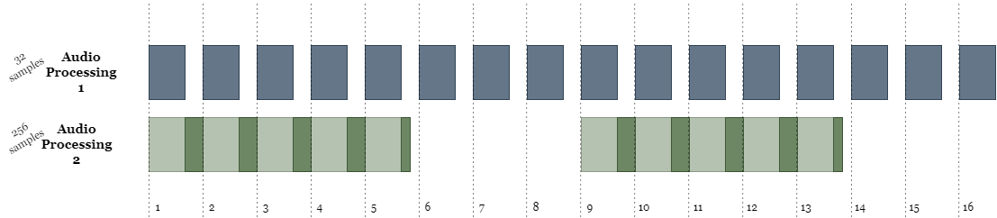
The 32 sample block processing, shown in dark blue, occurs at a uniform rate. While this higher priority processing is active, the 256 sample thread can not process and sits idle (light green) until the 32 sample processing is complete. When the 32 sample processing is not active then the 256 sample processing has a chance to execute, shown in dark green. The 256 sample processing must complete before the next 8 blocks of 32 samples arrive, or the system will be overflowed and audio will be dropped or corrupted.
In addition to Buffer Up/Down modules, all source modules, which are defined as any module that does not contain an input pin but does generate an output, can also control which clockDivider they belong to. To extend the Buffer Up → SOF → Buffer Down system described above, you can also add a sine wave to the buffered up audio signal as shown below:
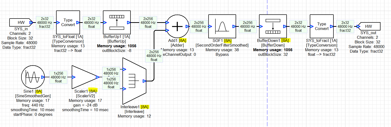
Example multirate system with a source module
Here, the all the highlighted modules are processing at the 1/8th block rate. To achieve this system, the clockDivider field of the Sine1 module must be set to ‘8A’ in the Build tab of the Module Properties menu. All the modules downstream of the Sine1 module will then inherit this clockDivider and run at that same block rate.
Multithread Processing
Some systems are able to run multiple threads or processes in parallel. For example, a quad-core Cortex A target may be able to assign individual threads to execute on different CPU’s, allowing them to be processed concurrently. In systems that can support this type of processing (see the AWE Core OS product), the Buffer Up V2 and Buffer Down V2 modules can be used to create new sublayouts without having to change the block rate of the processing.
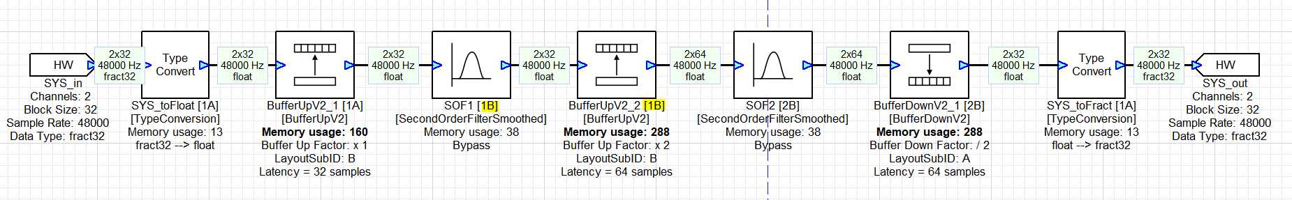
A multithreaded and multirate example system
In the layout above, the first BufferUpV2 module does not change the block rate / clockDivider of the downstream modules. It only changed the LayoutSubID, expressed as a letter, from A to B. This means that the downstream SOF1 module is going to execute at the same block rate (32 samples at 48 KHz) as the upstream modules, but that a new sublayout will be generated. This new sublayout can then be executed by the application on a separate core in order to maximize the processing power used on the target system without introducing the additional latency caused by changing the block rate. Up to 16 unique LayoutSubID’s (A through P) can be created for each block rate.
The next BufferUpV2 module does change the block rate by a divider of 2, so that the SOF2 module runs with a clockDivider of 2. The BufferDownV2 module buffers the system back down to the original 1A sublayout, which is then sent to the output pin. The module(s) that feeds the output pin must always have a clockDivider of 1, but the LayoutSubID can be any value.
Advanced users can generate an AWS from the layout above and observe that there will be 3 create_layout commands, one for each of the 1A, 1B, and 2B sublayouts:
0,create_layout,theLayout_1A,1,4
0,create_layout,theLayout_1B,1,3
0,create_layout,theLayout_2B,2,3
Similar to multirate processing, all source modules can also be configured to run on a specific LayoutSubID by modifying the clockDivider property on the Build tab of the Module Properties menu.
Limitations
One feature of Audio Weaver is that the smallest possible block time in the system corresponds to the fundamental block size of the target system. This means that the smallest block time in the layout occurs at the input pin of the system. Audio Weaver buffers can only BufferUp to larger block times from the input block rate. When using a platform with a fundamental block size of 32 samples, it is not possible, for example, to BufferDown to a 1 sample block size for stream processing.
Not all targets support multiple block rates, depending on the system and how the application is designed. The Threads field reported in AWE_Server while connected to the target reflects the possible number of different block rates that the target can support. Refer to the user guide of the specific hardware target to see if this feature is supported.