
SPL Meter
About This Guide
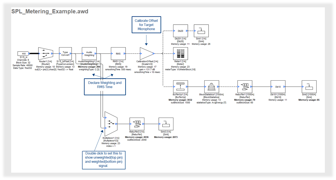
The SPL meter guide includes instructions for using the SPL_Metering_Example.awd which demonstrates concepts of audio weighting, smoothing with RMS, and converting between dBSPL and dBFS including some best practices for viewing signals in real time. It can be found within your Audio Weaver installation, in the “Examples” folder.
Audio Weighting
Audio weighting is used to account for the relative loudness perceived by the human ear at different levels.
· A-weighting emphasizes the speech band and ignores low frequencies
· C-weighting includes low frequencies
There can be a significant difference between measurements taken with A versus C weighting, especially if the source content contains lots of low frequency content (bass notes, road noise, etc.)
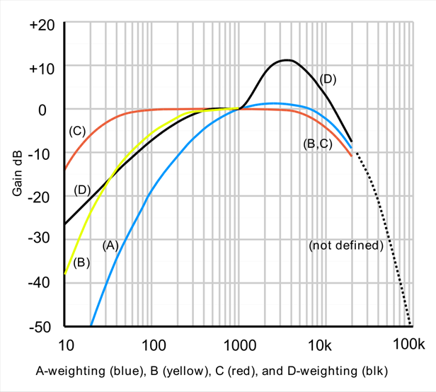
Figure 1 – Audio Weighting
Best Practices
· Use A-weighting when verifying microphone specifications, as this is the weighting used when manufacturers write the specs.
· Use C-weighting when doing Voice UI level measurements. C- weighting reflects how hard the algorithm has to work.
The following figures reflect different representations of white noise when various weighting is applied:
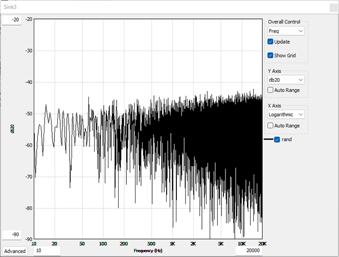
Figure 2 - Flat Weighting
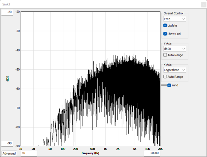
Figure 3 - A Weighting
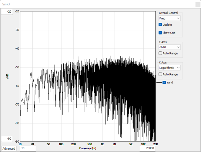
Figure 4 - C Weighting
RMS
The RMS module calculates the smoothed RMS value of the input signal on a block-by-block basis.
For each block, the sum of the square of all input data is computed (the energy), and this includes all channels and the entire block. Next, the energy is divided by the number of samples to yield the average energy. The average energy then passes through a first order lowpass filter with a specified integration time (the smoothingTime). Finally, the square root of the filter output is computed and this serves as the output of the module.
The module also exposes some of the computed signals as state variables. The variable filteredValue holds the output of the module (the smoothed RMS value). The variable instantaneousValue holds the square root of the average energy in the block; no smoothing.
Viewing the signal
Once the RMS is calculated, the design uses a dB20 module to convert from linear amplitude units to decibels, allowing us to view the smoothed signal as dbFS.
To graph the input signal over time with a Sink module, a BufferUp module is used to create a larger sample block to then create an average using the BlockStatistics module. Blockstatistics outputs a single sample block size, so that must be converted back to a larger block size in order to draw a graph. The design then converts from energy to decibels using a dB10 module (since we are transforming a quantity that relates to energy, not amplitude) and outputs to a SinkDisplay.
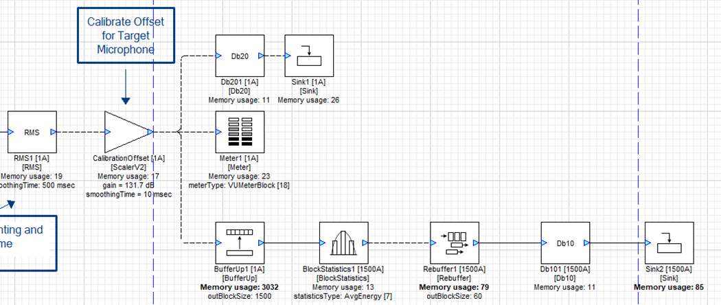
Figure 5 – Viewing the signal
Decibels relative to Full Scale vs. dB SPL
dB relative to Full Scale
When an analog microphone signal is converted to digital, units of decibels are represented as decibels relative to Full Scale, where 0 becomes the maximum output signal before digital clipping occurs, therefore all peak values will be negative numbers. For example, a signal that reaches 50 percent of the maximum level would be represented as -6 dbFS and so on.
Calibrating for SPL
When measuring source content with a microphone, it is necessary to convert from dbFS to dbSPL or vice versa in order to understand what the acoustic Sound Pressure Level would be to human hearing. To make this conversion, we must calibrate the microphone with a known reference level.
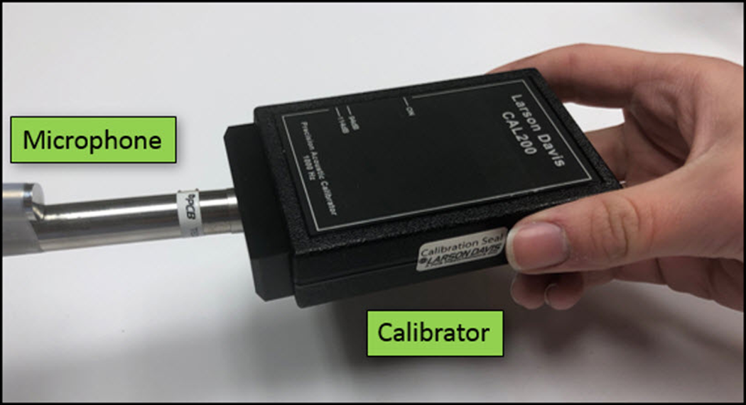
Figure 6 – microphone and calibrator (credit: https://support.sw.siemens.com )
How to set the dB offset
In the SPL_Metering_Example.awd there is a calibration offset scaler which should be adjusted so the dbFS reading on a meter module while the calibrator is connected to the microphone equals the sensitivity of the microphone.
For example, most calibrators will emit a 1000Hz tone at 94dB SPL, which is the reference level used when a manufacturer calculates a microphone's sensitivity. Therefore if a microphone's sensitivity is listed as -26dB, that translates to 94dBSPL. 1000Hz is used since it is a frequency that is unaffected by different weighting. Once calibrated, we know that if the meter reads -26dB, it is equal to 94 dbSPL.
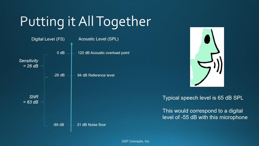
Figure 7 – Comparing dBFS and dBSPL