Generalized Cross Correlation Direction of Arrival Estimator
Introduction
Generalized Cross Correlation Direction of Arrival (GCC) utilizes frequency domain cross correlation to estimate time difference of arrival, (TDOA), between each set of microphone pairs for a given mic geometry. TDOA information for all mic pairs is then combined to estimate direction of arrival, (DOA) of one or more sound sources.
We pre-compute and tabulate TDOA vs DOA for each mic pair, based upon our knowledge of mic geometry. These lookup tables are used to help us form our DOA estimate.
We first compute frequency domain cross-correlation for each set of microphone pairs. We normalize this data and eliminate bins below mic noise floor. Next we zero pad the frequency domain data and take IFFT to get time domain cross correlation. The zero padding increases our time domain resolution. The time domain cross-correlation data will have peaks at index values corresponding to TDOA between that mic pair. We use the time domain data from all mic pairs to compute the best estimate of DOA.
We have made several improvements over the original GCCV1 module. The current module is known as GCCV7. We will first go over all the details of the basic GCCV1 module and then describe the improvements made for GCCV7.
Generalized Cross-Correlation Calculation
The meat of the GCC DOA calculation is the cross-correlation calculation between all microphone pairs. The output of the generalized cross-correlation is the similarity between two microphone signals as a function of time-lag. Based on this information and the known microphone geometry, the direction of arrival can be estimated. See later sections for how this is performed.
Generalized Cross-Correlation with Phase Transform
The calculation for this is as follows:
Where Xi and Xj are two microphone signals and i is not equal to j. Epsilon is a very small number preventing division by zero. This calculation is done on a bin-by-bin basis. Dividing by the magnitude has the effect of 'whitening' the signal, i.e. giving an equal contribution for all frequency components. This will give us a more distinctive peak in our time domain correlation function. G is the GCC-PHAT coefficient. PHAT refers to the Phase Transform, which is the denominator of the equation above. G is a complex-valued vector.
GCC-PHAT Coefficient Weighting
One issue that GCC-PHAT does not address is the presence of the microphone noise floor. The denominator of the equation above will normalize the magnitude of each of the frequency bin to unity, which means that only the phase of each frequency bin is relevant. This works well if the input signal has high energy in all frequency bins relative to the noise floor of the microphones. In reality, if the input has no content in a frequency bin, then the phase of that bin is the random phase of the noise floor. If the signal level is roughly the same level as the noise floor, then the phase information will be somewhat contaminated by the noise floor. To solve this issue, a new weighting scheme needs to be created so that the magnitude of the frequency bin is weighted by the signal to noise ratio.
The Wiener solution is the linearly optimal weighting for this scheme:
where S is the variance of the signal and N is the variance of the noise. W is the weighting. This is a real-valued vector which has the same length as the number of frequency bins.
S is measured from the real-time microphone data. N is the pre-measured noise floor of the system. This can be done with the same methodology has the noise floor adjustment in our Max SNR Beamformer design.
In practice, the above equation is modified to be more tunable and more easily understandable:
Sdb is the measured signal level in dB. Ndb is the measured noise floor level in dB. bdb is the user tuned parameter, in dB, to adjust the weighting curve.
Essentially, the weighting function is a sigmoid function based on the level difference between the microphone and the measured microphone noise floor (pseudo-SNR estimation). The user tunable b value shifts the sigmoid to the left or to the right.
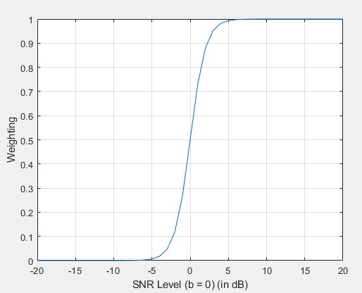
The weighting as a function of the SNR level with b = 0.
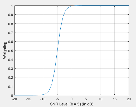
As the b value goes up, the more tolerant the system is to microphone noise.
A noise floor measurement is recommended over a single noise floor value over all frequencies because the microphone noise floor is highly dependent on frequency. Below is an example of a real-world microphone noise floor measurement:
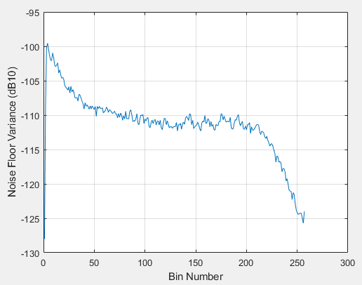
The noise floor levels vary as much as 20dB+. This will drastically affect the weights based on the wiener solution above.
The GCC-PHAT coefficients are weighted with this weighting:
Where the circle-dot operation represents element-wise multiplication.
Future Improvements - if precedence logic is needed, then the weighting function can be extended to include this.
Interpolation and IFFT
To get the time delays, the weighted GCC-PHAT coefficients are transformed with an inverse Fourier Transform operation. However, by performing the IFFT operation on the GCC-PHAT coefficients as is, the time-delays are quantized to the nearest sample. If the input time-domain signal is 16kHz then each sample represents 62.5 μs. Then, assuming the speed of sound to be ~343 m/sec, each sample in the time-delay represents 21.5mm. And so, by performing this operation at 16kHz, and the spacing between two microphone pair is 75 mm, then allowable delays are [-3, -2, -1, 0, 1, 2, 3], which is only 7 discrete values. This is a very bad resolution for a decently sized microphone array.
To solve this, interpolation between the samples are needed. If a more reasonable range, say 49 discrete values, is desired, then time-delay should be upsampled by a factor of 8. The most efficient way to upsample is by zero-padding the GCC-PHAT coefficients before the IFFT operation. To upsample by 8, the original GCC-PHAT coefficient should be zero-padded with 7x its original length. An IFFT operation is then performed on this zero-padded GCC-PHAT coefficients so that in the time-delay signal is now at a higher sample rate than the original. If the original sample rate is 16kHz and the interpolation factor is 8, then the time-delay signal is now at 128kHz. Each sample in this now represents ~8 μs or 2.7 mm, giving a much higher resolution.
The GCC-PHAT coefficient to Time-Delay transform should be done with a pure IFFT operation, not WOLA Synthesis. The reason is that the WOLA Synthesis time-aliases the current samples along with a few previous blocks of samples. This effectively causes smearing in the time axis of the Time-Delays, leading to worse estimation. The GCC AWE module performs the IFFT operation internal with a call to the AWE IFFT module, (ifft_module).
Time Difference of Arrival to Direction of Arrival Mapping
Taus(theta) Function
The expected delay as a function of angles of arrival for a microphone pair is precomputed based on the microphone geometry. We will refer to this function as Taus(theta). For example, given the microphone geometry below:
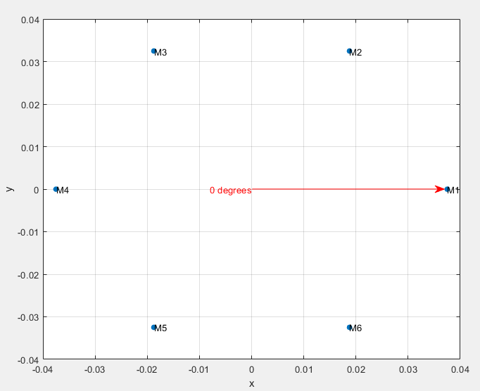
Taus(theta) for microphone pair 1 (time delay between mic 1 and mic 2) is shown below.
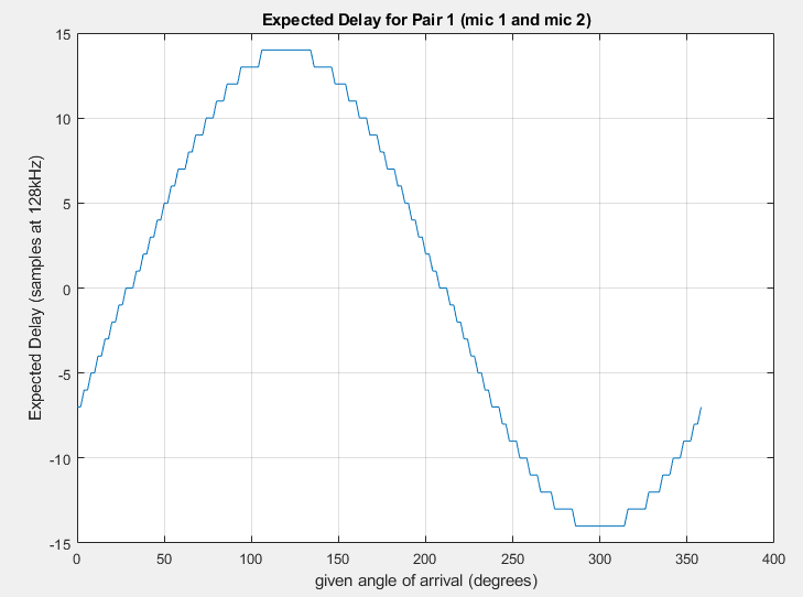
Notice that:
The time delay is 0 samples at 30 degrees and 210 degrees. This corresponds to when the sound source is exactly at broadside to the microphone pairs.
The time delay reaches its maximum and minimum at 120 degrees and 300 degrees respectively. This is the end-fire orientation to the microphone pairs. The max and min values of Taus(theta) for a given microphone pair is based on the distance between the two microphones, the speed of sound, and the sample rate of the system.
Except for the end-fire directions, each time delay corresponds to two potential angles of arrival. This is the front-back ambiguity for a linear microphone array.
Due to the microphone spacing and the sample rate, there is quantization of expected delay vs the angle of arrival. For example, angles of 28-32 degrees correspond to an expected delay of 0 samples. Likewise for angles 208-212. In other words, if the measured delay is 0 samples and the angle of arrival is limited to between 0 and 180 degrees (based on other cues). Then based on this microphone pair alone, the possible angles of arrivals are 28, 29, 30, 31, 32 degrees... which has a resolution of about 4 degrees.
The quantization of expected delay is not uniform across all angles. At the end-fire orientations, the quantization is at its worst. At an expected delay of 14 samples, the valid angles of arrival are between 106 and 134 degrees. The angular resolution is approximately 28 degrees.
The angular resolution is related to the derivative of Taus(theta) with respect to the angle of arrival. Taus(theta) is a sine function, and so the derivative is just a 90 degree shifted version. Which means that at the extremes, the derivatives are very small, so the angular resolution is poor. The greatest derivatives are at the 0 crossings of Taus(theta). Hence the 4-degree resolution at 30 degrees angle of arrival.
The angular resolution affects the performance of the DOA estimation. The finer the resolution, the greater the ability to pinpoint the source as well as reducing the variance of the error. There are a few ways achieve greater angular resolution, all with different tradeoffs:
Increase the sample rate of the microphone. This will allow finer capture of the sound at the expense of increased system costs.
Increase the interpolation factor. This is essentially doing the same thing as #1 without the increase of hardware cost. However, the greater the interpolation factor, the more aliasing is likely to happen. (?????)
Increase the microphone spacing. This will also give a greater delay between samples. But this can introduce spatial aliasing which can affect the cross-correlation calculation.
Depending on the microphone array geometry, there typically could exist at least another pair of microphone that has a finer resolution at an angle than another pair. The plot below is the Taus(theta) function for two microphone pars - M1, M2 pair and M1, M6 pair. Based on the microphone geometry, these two microphone pairs are especially complementary to each other. This is because of the fact that the broadside angle (the best angular resolution) of one pair is very close to the end-fire angle of the other pair (the worst angular resolution).
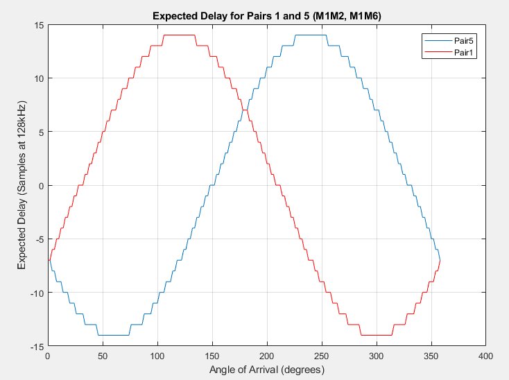
Notice that:
At the worst angle for pair1 (106 to 134 degrees), this corresponds to almost the best angle for pair 5. For pair 1, angles 106 to 134 corresponds to a single delay (14 samples). For pair 5, these angles correspond to 6 different delay samples: -10 samples to -4 samples.
This is also true for the worst angle for pair5 (46 to 74 degrees). In this region, pair 5 has a single delay sample, but pair 1 spans 6 different samples.
Future improvements:
Given the idea that the angular resolution is different depending on the angle of arrival, it is possible to design an optimal weighting function that'll weight the contribution of the measurement based on the theoretical angular resolution.
Trimming Down Time Domain Cross Correlation Function Using the Taus(theta) Function
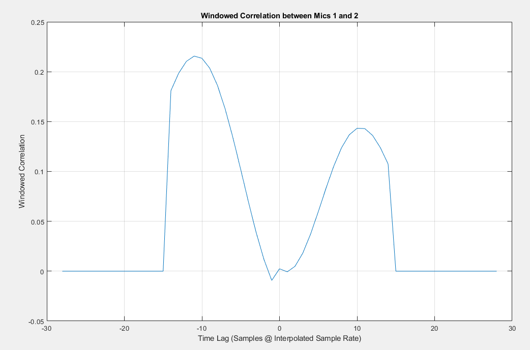
After taking IFFT of the zero padded GCC-PHAT data we get the time domain cross-correlation for a given mic pair. An example of the cross-correlation measurement is below. This is the cross-correlation measurement of microphones 1 and 2 with the microphone geometry above:
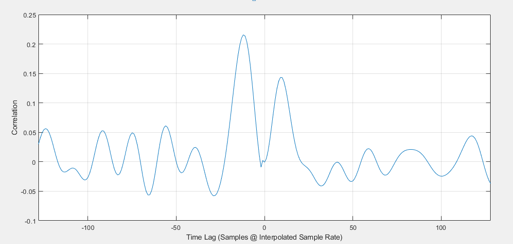
The interpretation of this chart is as follows. For two given microphone signal, one of the microphone signals is delayed and the dot product is computed. The x-axis represents the amount of delay in samples and the y-axis represents the value of this dot product. The dot product is a measure of similarity between two vectors - the greater the value - the greater the similarity. A value of 0 means there is no similarity between the two signals. Therefore, any peaks in the correlation value suggest a similarity in the signal at that time lag.
The time lag corresponds to the "Expected Delay" of the Taus(theta) function. And so, depending on the microphone pair and the measured correlation at each time lag, the Taus(theta) function will map the correlation value to an angle of arrival.
Note that depending on the microphone geometry, there is a maximum and minimum possible time lag. This corresponds to the max and min value of the Taus(theta) function for this microphone pair. In this instance, the microphones 1 and 2 has a maximum time lag of 14 samples and minimum time lag of -14 samples. Any correlation values beyond this limit could be residuals from the cross-correlation estimation, certain aliasing effect, or reflections captured within this time block. In any case, these values are considered junk and are discarded.
The windowed generalized cross-correlation is generated based on the observation above:
Future improvements:
There can be different windowing of the Windowed GCC function such as a sliding max window. This window could potentially improve the variance of the estimation but decrease the angular resolution
Potentially possible to do a gating of the GCC values... for example, any GCC value that's below a threshold is set to 0.
Calculating Direction of Arrival
The algorithm has 2 main steps. Each step is performed once for each WOLA block.
Step I.)
For Each Mic Pair:
1.)Compute Cross Correlation in Frequency Domain
2.)Divide Correlation by its magnitude, (PHAT weighting)
3.)Zero out noisy bins in GCC-PHAT
4.)Zero pad GCC-PHAT to increase TD resolution. Amount of zero padding is specified by module argument 'interpFactor'
5.)Perform IFFT giving us Time Domain Correlation
6.)Trim TD Correlation to lags possible for this mic pair.
Step II.)
//Sum(Angle) is an array of 360 float values
Set Sum(Angle) to all zeros
For Each Angle, (0-359)
For Each Mic Pair
{
1.)Look up lag for this angle in Taus(Theta)
2.)Get TD Correlation value for this lag
3.)Add TD Corr value to Sum(Angle)
}
DOA Angle Estimate = argmax(Sum(Angle))
At the end of Step II we have the Sum(Angle) array with 360 values. The maximum value of this array represents the sum of the cross correlation functions for all mic pairs for a direction of arrival at this value of Angle. We can use this Sum(Angle) array to report estimates of multiple sources. Multiple sources are reported as the peaks in this array. However we have logic to prevent us reporting 2 sources which are too close together.
It is somewhat intuitive that the peak of the Sum(Angle) array represents the best estimate of DOA. To make this more clear, it is possible to prove that the peak of the Sum(Angle) array is mathematically equivalent to the angle giving max power for a DAS beamformer of the same mic geometry. i.e. consider a DAS, (Delay and Sum), beamformer using the same mic geometry which takes our data for this WOLA block as input. Then consider changing the look direction of the beamformer over angles from 0 to 360 and looking at the output power of the beamformer. We can show that the angle with max power output from the beamformer will always be the maximum of the Sum(Angle) array. The 2 are mathematically equivalent that way. They are not mathematically identical but equivalent in that the same angle gives max value for both.
Zeroing out noisy bins
The array noiseFloorVar[ ] contains microphone noise floor measurements/estimates per bin computed or measured offline. The module variable noiseFloorDBOffset contains a user selected value for noise floor weighting. Let CC(bin) = the complex frequency domain cross correlation value. Let M(bin) = the magnitude of CC(bin). Let MdB(bin) = M(bin) in dB10 units. We compute GCC-PHAT(bin) as:
diff = MdB(bin) - noiseFloorVar(bin);
delta = diff + noiseFloorDBOffset;
doaWeight = 0.1666667 * delta + 0.5;
if(doaWeight < 0)
doaWeight = 0;
if(doaWeight > 1.0)
doaWeight = 1.0
GCC-PHAT(bin) = (CC(bin)/M(bin))*doaWeight;
Improvements made for GCCV7
Summary:
1.)Eliminate dB10() Function Calls
2.)Allow Using a Subset of WOLA Bins, (precede with Block Extract module)
3.)Time/Frequency Domain Smoothing of Input Data
4.)Quadratic Interpolation
5.)Combine Congruent Mic Pairs
6.)Histogram Processing
Details:
1.)Eliminate dB10() Function Calls
Original code stored the noise floor array in linear units and then each WOLA block converted to dB10 with calls to the dB10() function! Now we store the noise floor array in dB10 units and avoid the conversion.
2.)Allow Using a Subset of WOLA Bins, (precede with Block Extract module)
Original code required that all WOLA bins be input to the module and processing was done for all bins. Now we allow processing on a subset of the WOLA bins by preceding the GCCV7 module with a Block Extract module. This can save us MIPS and also allows us to get rid of bins which have frequencies that are too low or too high to accurately estimate DOA. Frequencies which are too low have more acoustic noise and also have wavelengths which can be too long relative to the mic spacing. Since the algorithm works on phase difference, low frequency/long wavelength bins have phase differences which are too small to make any meaningful estimate of DOA. Frequencies which are too high can have spatial aliasing. In this case freq 1 at angle 1 and freq 2 at angle 2 can appear identical in terms of phase shift and so we can get errors in estimating DOA.
We have a new module parameter LowerBin which must be set correctly to match the lower bin of the Block Extract Module. This is necessary since the module cannot determine this information from its input wires.
The module's MIPS consumption is roughly proportional to the number of bins the module processes. We can reduce the number of bins processed further to save MIPS, but this will possibly decrease accuracy. The user must experiment with this for their own application. We must always give the module a contiguous range of bins. Internally the module expects this and will not work correctly if this condition is not met. LowerBin variable must always be set to match the lowest bin entering the module.
3.)Time/Frequency Smoothing of Input Data
We can increase accuracy of GCC by doing smoothing/averaging on our correlation data. This smoothing may be performed either in the frequency domain or in the time domain. If we do the smoothing in the frequency domain we operate on the GCC-PHAT data before taking the IFFT. If we do the smoothing in the time domain we operate on the trimmed time domain correlation data. We do exponential smoothing of the data. Let SC denote our 'smoothing coefficient'. Then our smoothing equation looks like: state(n) = SC*(new data) + (1-SC)*state(n-1). We are doing the smoothing on the data for each mic pair.
The value of the smoothing coefficient allows us to trade off accuracy and responsiveness. SC can vary between 0 and 1. The smaller the value of SC the longer the tail of our exponential smoothing/averaging. If SC == 1 we are doing no smoothing. Doing more smoothing gives us more accuracy but less responsiveness and vice versa. The smoothing coefficient is a live tunable variable. We may also take our smoothing coefficient from an optional input pin. This allows us to dynamically control the degree of smoothing based upon knowledge of our signal environment. This is selected via the useSmoothingPin module argument.
If we do frequency domain smoothing then we need numSB*numMicPairs complex values for state array. If we do time domain smoothing we need only one smaller state array of size tdLength float values. Where tdLength is the size of one trimmed correlation function. So for memory savings we prefer using time domain smoothing. However time domain smoothing can only be done if we are only reporting one DOA estimate. The module's constructor automatically selects time versus frequency smoothing correctly based on the module arguments: smoothing, maxNumSources, useSmoothingPin. The smoothing and useSmoothing can take on values of 0 or 1. maxNumSources specifies how many distinct audio directions to estimate. The logic used is:
if((useSmoothingPin==0) && (smoothing==0))
smoothingTyoe = 0; //No Smoothing
elseif(maxNumSources==1)
smoothingTyoe = 2; //Time Domain Smoothing
else
smoothingTyoe = 1; //Frequency Domain Smoothing
4.)Quadratic Interpolation
This is performed on the trimmed time domain correlation data. Quadratic interpolation is always performed. This allows us to do less zero padding of the frequency domain GCC-PHAT data, and thus do smaller IFFT's, and still get the same accuracy. Quadratic interpolation takes less MIPS than a larger IFFT. Quadratic interpolation is performed in the 2nd step of the angle estimation algorithm:
Step II.)Including Quadratic Interpolation
//Sum(Angle) is an array of 360 float values
Set Sum(Angle) to all zeros
For Each Angle, (0-359)
For Each Mic Pair
{
1.)Look up lag for this angle in Taus(Theta)
2.)Get TD Correlation value for this lag, and its 2 adjacent lags
3.)Perform quadratic interpolation using these values to obtain more accurate TD Corr value
4.)Add TD Corr value to Sum(Angle)
}
DOA Angle Estimate = argmax(Sum(Angle))
5.)Combine Congruent Mic Pairs
For some mic geometries we can save MIPS by eliminating redundant mic pairs from most of our computations. This option is selected with the module argument: 'combineCongruentMicPairs'. We will usually set this to 1. Only reason to set this to zero would be for debugging. For a mic pair MiMk we can define a vector between the 2 mics. We will call this vector Vij. 2 mic pairs, Mij, and Mkl are congruent if Vij and Vkl are identical or if they have identical magnitude and opposite directions. When we set combineCongruentMicPairs to 1, then the code automatically only performs the Step II processing on the non-congruent mic pairs. Some of the Step I processing is still done for all pairs. We average the frequency domain GCC-PHAT data for all sets of congruent pairs. This gives us a better estimate of the frequency domain generalized cross correlation. However we do the Step II processing only on the averaged GCC-PHAT data for the redundant mic pairs. This saves us doing IFFT's on the redundant mic pairs. This gives significant MIPS savings as the lion's share of the MIPS are used in IFFT calculations.
6.)Histogram Processing
GCCV7 produces an estimate of DOA every WOLA block. A typical block size is 5ms. We found that our output data was fairly noisy. We tried several averaging methods to fix this without good results. We settled on histogram processing to smooth out the noisy data. We accumulate angle estimates over a selected number of blocks into a histogram. The histogram is an integer array indexed 0-360. Each WOLA block we add our angle estimate to the corresponding histogram entry. Then after we have accumulated the selected number of blocks we output the indices/values of the histogram peaks. We can output one or more peaks corresponding to one or more DOA's. The histogram processing is found to produce much cleaner and more accurate angle estimates. We have a live tunable parameter, ('BlocksPerHistogram'), which selects the number of WOLA blocks to accumulate into our histogram. So if we have 5ms blocks and BlocksPerHistogram = 128, then our accumulated histogram spans 640ms.
We do further processing on the histogram data: the module argument NumHistogramStates selects the number of accumulated histograms to average together before producing output. Thus if we have 5ms blocks, BlocksPerHistogram = 128, and NumHistogramStates = 4. Then we are using information over 2.56 seconds. We produce new output every BlocksPerHistogram, (640ms), but each new output is the average of the current 640ms block with the previous 3 640 ms blocks. Finally we do gaussian smoothing of the averaged histogram to clean it up and make it easier to pick out the peaks. There are 4 more live tuning parameters related to histogram processing:
doHistSmoothing
Checkbox to turn histogram smoothing on and off
doHistAveraging
Checkbox to turn histogram averaging on and off
MinPeakThresh
Float value to select the minimum value of a peak to be considered a valid angle estimate
MinDist
Integer to select the distance in degrees between 2 histogram peaks to be considered seperate peaks/angle estimates