
Make a Convolution Reverb using the Long FIR Module
About This Guide
This document describes using the Long FIR module to achieve improved (reduced) CPU utilization when processing very long FIR filters. The specific application described is a convolution reverberator.
Introduction
FIR filters, while very flexible and convenient to use, can take a lot of CPU cycles to process, if they are very long. The number of calculations required to process a single sample goes up as the square of the length of the filter in samples. So, a FIR filter with 100 coefficients will require 4 times as much processing as one with just 50 coefficients.
The Long Fir module improves on this by using a method known as FFT Convolution. Rather than needing N^2 computations per sample, only N * log2(N) computations are needed. The larger N is, the better the savings in CPU cycles. The tradeoff is an increased use of RAM.
This example requires the use of AWE Designer Pro as we use a MATLAB script to process the impulse response (IR) WAV file and upload the coefficients to the Long FIR Modules.
Reference Data Set
We will use data from two WAV files representing the impulse responses of
the Cathedral Room at Shasta Lake Caverns in California.
http://www.echothief.com/cathedral-room-shasta-lake-caverns/
WAV file with 67,421 samples at 44.1 kHz sampling rate
Battery Benson, Jefferson County, Washington.
WAV file with 80,271 samples at 44.1 kHz sampling rate
By using the FIR block to process input audio with the data from these WAV files, we will create a “Convolution Reverb” that makes your audio sound like it would in the physical space.
Baseline Performance using the FIR Module
Load the file “ReferenceFirExample.awd” into AWE Designer. The FIR Block already contains the coefficients from the left side of the stereo WAV file representing the cavern’s impulse response.
Running this program gives the following results on a Windows 10 PC with the following specs:
AMD Ryzen 5 2600 CPU @ 3.40 GHz
16 GB RAM
AWE Server display:
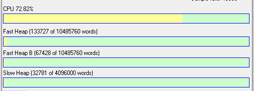
Figure 1. Performance with FIR Module
Using the Long FIR Module
The steps needed to use the Long FIR module are:
Place the following files in the same folder.
CathedralReverb.wav
BatteryBenson.wav
format_long_fir_coeffs.m format_long_fir_coeffs.m
LongFIRExample.awd LongFIRExample.awd
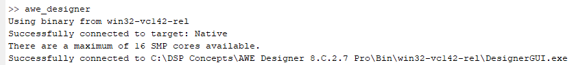
Open MATLAB and run “awe_designer” at the command prompt.
Open LongFIRExample.awd in AWE Designer.
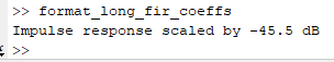
Open the format_long_fir_coeffs.m script in MATLAB
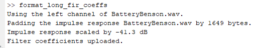
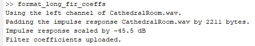
Run the script to process the cavern impulse response WAV file and load the coefficients of the 3 Long FIR modules. You will see the following output, which indicates that the coefficients were scaled down by 45.5 dB. This helps to prevent distortion in the filters. The actual value you see will depend on the WAV file being used.
Now run the LongFIRExample1a.awd in AWE Designer. Here is the performance, along with a table comparing these results to the previous example which used the regular FIR module.
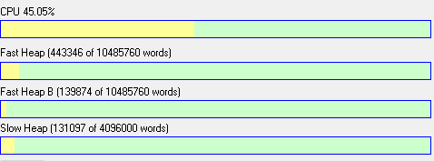
Filter | CPU | Fast Heap | Fast Heap B | Slow Heap | Total RAM |
FIR | ~73.0% | 133727 | 67428 | 32781 | 233,936 |
Long FIR | ~45.0% | 443346 | 139874 | 131097 | 713,217 |
As you can see, using the Long FIR module achieves a roughly 28% saving in CPU cycles at the expense of using about 3 times as much RAM on this PC. The actual differences in performance and RAM usage will depend on the actual device running the program.
Using the Long FIR module in your own designs
Let’s take a look at the example patch. The input signal is sent to three parallel processing paths, identified as “First Chunk”, “Second Chunk” and “Third Chunk”.
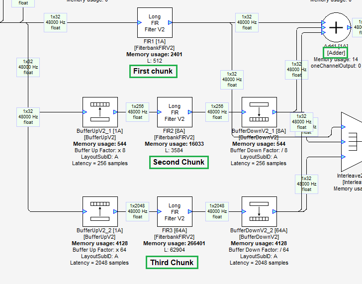
The impulse response WAV file has been broken into 3 chunks by the MATLAB script, matching the size of the data to the length (in taps) of each filter. The audio data goes directly to FIR1 which is implementing the first chunk of the impulse response (512 taps). The subsequent Long FIR Filter V2 blocks need to have BufferUpV2 blocks added to increase the size of data that is being processed at one time. Here’s how to do it. (The supplied LongFIRExample.awd file implements this).
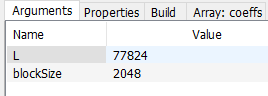
Set the length (Argument “L”) of the first Long FIR module to 512.
In the BufferUpV2 block for the second chunk, adjust the BufferUpFactor to be 512/2 * (input pin block size). In this example that is 512/(2 * 32) = 8.
Set the length L of the FIR2 module to an integer multiple of the FIR1 module’s length. In this case we have used 512 * 7 = 3584.
Note that the total length of FIR1 and FIR2 is 512 + 3584 = 4096.
In the BufferUpV2 block for the third chunk, adjust the BufferUpFactor to be 4096/2 * (input pin block size). In this example that is 4096/(2 * 32) = 64.
The length of FIR3 is determined by taking the total length of the first two chunks and subtracting that from the total length of the impulse response’s WAV file in samples. In this example, 67,421 - 4096 = 63,325. Now you need to round that to the next highest multiple of (FIR1 + FIR2)’s length. That is calculated as 4096 * (floor (63,325 / 4096) + 1) = 65536. We’ll add (65536 - 63325 = 2211) zeroes at the end of the data.
Running the MATLAB script
A MATLAB script is provided to manage formatting the impulse response data automatically. This includes:
Reading the WAV file into an array
If stereo, choosing the left channel
Breaking the WAV file data into chunks of 512, 3584, and “the rest” (samples).
Zero-padding the last chunk so that its length is an integer multiple of the sum of the first two (512 + 3584 = 4096).
Uploading the chunks to the individual filter modules in the LongFIRExample.awd file.
To run the MATLAB script:
Place the LongFIRExample.awd file, the MATLAB format_long_fir_coeffs.m file, and the two impulse response WAV files in the same folder.
Open the MATLAB application.
At MATLAB’s console, run: awe_designer
When AWE Designer opens, load the LongFIRExample.awd design file.
In MATLAB, open the format_long_fir_coeffs.m script.
Confirm that the designerFile and reverbImpulseRespWav variables are set correctly.
Run the MATLAB script.
If you see this message:

then open the Properties panel of FIR3 in AWE Designer, and set the “L” argument to the value shown.
Run the script again. It should complete without any error. Note that the results for the two WAV files are slightly different.
Reconstructing the filter response
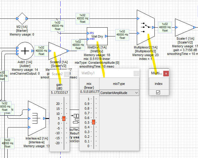
The output of FIR1 goes to the first input of Adder Add1.
The output of FIR2 goes through a BufferDownV2 block and then to the second input of Add1.
The output of FIR3 goes through a BufferDownV2 block and then to the third input of Add1.
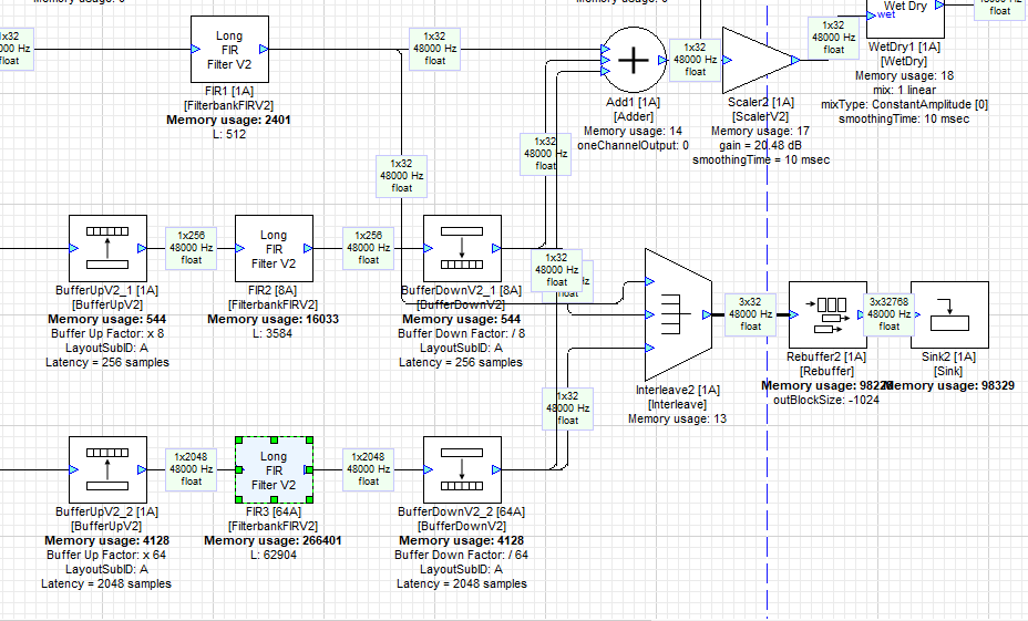
This design also interleaves the 3 signals onto a single wire and sends them through a Rebuffer module and onto a Sink, so that we can see that the impulse response has been reconstructed from the 3 separate filters and properly time aligned. The Interleave, Rebuffer, and Sink modules are not needed other than to see this and can be omitted from your own designs.
The Multiplexor1’s index checkbox has been selected, so that we are feeding impulses from ImpulseMSecSource1 to the filter. This allows you to check both the basic sound of the reverb and visually compare the reconstructed impulse response with the original signal.
Run the patch, then click on “Sink2” to open the waveform display.
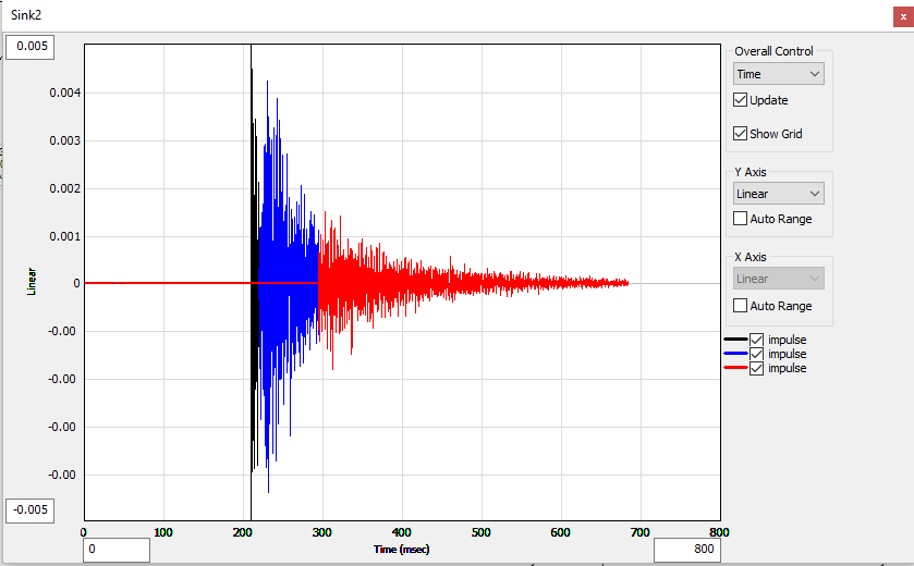
You can see by the colors that the composite impulse response has been reconstructed by adding the 3 signals together.
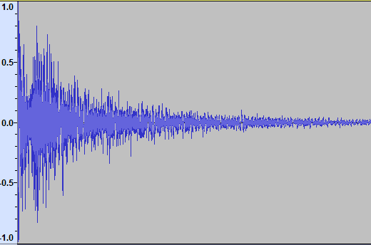
For comparison, here is the waveform view in Audacity of the original WAV file.
Signal Mixing and Bypass
Scaler2 allows you to adjust the level of the reconstructed reverb signal. This feeds into WetDry module WetDry1, which lets you set the balance between the dry (input) signal and wet (reverb). At a setting of 0, you just hear the dry signal. At 1.0, you only hear the reverb signal.
The MultiplexorV2 Multiplexor2 implements a bypass function. When the index checkbox is selected, the reverb is engaged.
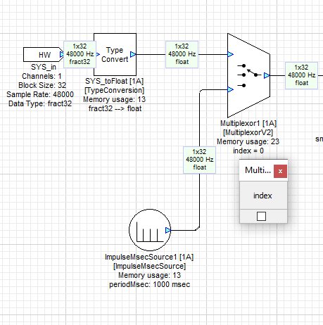
Input Signal Selection
Using the MultiplexorV2 Multiplexor1, you can select either the default signal source, or a series of impulses (clicks) that repeat once a second (if the index is checked). Impulses are a convenient and consistent way to test reverb algorithms.
Appendix A: MATLAB Script format_long_fir_coeffs.m
% This script file loads an impulse response stored in a WAV file, formats
% the coefficients, and then sends to Audio Weaver. Make sure that you
% have the file whose name is given by the designerFile variable open in Designer.
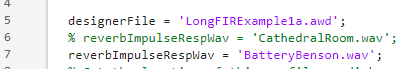
designerFile = 'LongFIRExample.awd';
% reverbImpulseRespWav = 'CathedralRoom.wav';
reverbImpulseRespWav = 'BatteryBenson.wav';
% Get the location of this .m file on disk
str = mfilename('fullpath');
ind = find(str == filesep);
dirStr = str(1:ind(end)-1);
LR = audioread(fullfile(dirStr, reverbImpulseRespWav));
GSYS = get_gsys(fullfile(dirStr, designerFile));
% Get the lengths of the individual filters
L1 = GSYS.SYS.FIR1.L;
L2 = GSYS.SYS.FIR2.L;
% make sure that the size of L3 is an integer multiple of L1 + L2
wavLengthInfo = size(LR);
wavLength = wavLengthInfo(1) - (L1 + L2);
L3Length = floor(wavLength/(L1 + L2)) * (L1 + L2);
% L3PadLength is number of zeroes to add so that L3 is an integer
% multiple of (L1 + L2).
L3PadLength = L1 + L2 - wavLength + L3Length;
% Zero pad or truncate the impulse response
% LR = truncate(LR, L_total);
L = LR(:, 1);
R = LR(:, 2);
% Pick which impulse response to use
fprintf(1,'Using the left channel of %s.\n', reverbImpulseRespWav);
h = L;
zeroes = zeros(L3PadLength, 1);
fprintf(1,'Padding the impulse response %s by %d bytes.\n', reverbImpulseRespWav, L3PadLength);
h = [h; zeroes];
% Scale the impulse response. Keep the peak frequency response value at
% 0 dB
p2 = ceil(log2(length(h)));
FFT_L = 2^p2;
H = desym(fft(truncate(h, FFT_L)));
Hmax = max(abs(H));
h = h / Hmax;
fprintf(1, 'Impulse response scaled by %.1f dB\n', db20(1/Hmax));
% Split into individual filters
h1 = h(1:L1);
h2 = h(L1+1:L1+L2);
h3 = h(L1+L2+1:end);
% Update the coefficients
GSYS.SYS.FIR1.coeffs = h1;
GSYS.SYS.FIR2.coeffs = h2;
% the argument FIR3.L in the awd file needs to be set manually for each
% impulse response WAV file. This try-catch code shows an error message
% if the size is not correct.
length3 = L3Length + L1 + L2;
GSYS.SYS.FIR3.L = length3;
try
GSYS.SYS.FIR3.coeffs = h3;
catch
warning('Make sure the that "L" argument of FIR3 is %d\n', length3);
return
end
% Now send the updated system to Designer
set_gsys(GSYS);
disp('Filter coefficients uploaded.');
Appendix B: References
Echothief Impulse Response Library
Fast convolution by FFT
Smith, J.O. "Fourier Theorems for the DFT", in
Mathematics of the Discrete Fourier Transform (DFT)
with Audio Applications, Second Edition,
http://ccrma.stanford.edu/~jos/mdft/Fourier_Theorems_DFT.html,
online book, 2007 edition, accessed 02/14/2023.