
Filters
This section contains the following pages:
Links to individual module pages can also be found in the table at the end of this page.
General Information
The Audio Weaver Filters folder lists over 60 filters. They have been broken down according to user needs, with the folder labels Adaptive, Calculated Coeffs, Controllable, High Precision, Raw Coeffs, and list the most commonly used filters. The Adaptive folder contains the LMS module, an adaptive filter with tracking capabilities. For those users less experienced with designing filters, the Calculated Coeffs filters take in frequency information, Q, Gain, and type, similar to tuning a filter in a DAW. Users with more DSP background can use the Raw Coeffs filters to tune filters with mathematical information. The most frequently used filters are the ButterworthFilter (highpass, lowpass, allpass), SecondOrderFilterSmoothed, with 20 different filter types, and the SecondOrderFilterSmoothedCascade: multiple 2nd order filters in series.
Adaptive (LMS)
The LMS filter predicts the FIR of a system whose transfer function is not given. It’s input and output adapt or “predict” what the system response is. Filter weights are updated over time based on mu speed, higher numbers being the faster update speed. Higher numtaps give higher chance to converge with the optimum filter weight(meaning less error). The error can be tracked realtime with the errorSignal output. The module comes with an option to output the predicted “coeffs”. The following system shows white noise being ran through a 10 point FIR. The LMS will predict the FIR coefficients, and sinks will display the error and coeff function.

This sink shows the coeff prediction.

The LMS is trying to predict this FIR response.
The Error2 display shows a value of -125 dB, which means that our signal is very accurate. The sink to the right displays this as well.
Filters with Calculated Coefficients
Audio Weaver has a several filters with built-in design equations. These filters are implemented using Biquad or BiquadCascade modules behind the scenes and the filter coefficients are computed by the design equations based on high-level filter specifications. The design equations use the sample rate on the input wire when computing coefficients. The following sections describe each of the calculated coeffs modules.
Allpass Pair
The Allpass Pair module creates a pair of allpass filters with the special property that their sum and difference form a doubly complementary highpass-lowpass filter pair. When used in conjunction with the Sum and Difference module (available in the Math folder) this Allpass Pair module can be used to construct more complex structures such as N-way crossovers and filter banks. The following design mixes one channel of white noise into two “bands” of white noise using this technique. The sink is an FFT showing the frequency response of the signal.

Audio Weighting Filters
The AudioWeighting module is located under Filters/Calculated Coeffs This module applies different standard audio weighting to a signal. The available weightings are selectable from the inspector and include: A, B, C, and D-weighting, as well as ITU468, LeqM, and ITU 1770. The WeightingFilter is used for noise measurements and broadcast loudness applications. The following frequency responses display each weighting’s filter.


Crossover Filter
A crossover is a special type of filter that splits a signal into multiple bands, while sustaining a total gain of 0 dB. It will boost the level of one frequency band as the other drops to compensate to 0 dB gain. This behavior is shown in the figure below.

Crossovers are used in loudspeaker applications to separate signals into different frequency bands to be output via woofers, mid-range, and tweeter speakers. They are implemented using ButterworthFilter (odd-order) or Linkwtiz-Riley (even-order) filters. Crossover filters can be made manually using individual filters. By cascading filters and applying an allpass filter during other lane filter stages (shown below), more crossover points can be added and the signal split into more frequency bands, while retaining the unity gain property.
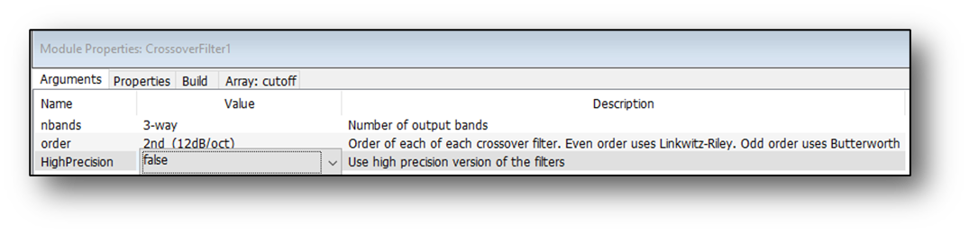
Alternatively, use the crossover module which contains all of the needed filters. The Crossover Filter module allows the user to set the type of filter, number of output bands, and filter order, specified in the module’s properties. Crossovers are used for separating different frequency bands of a signal. The example below demonstrates a crossover module being used to split a signal into a high band above 250 Hz and a low band below 250 Hz. The sum of the levels of the two bands is always 0 dB. As the input frequency changes near 250 Hz, one channel’s level drops and the other smoothly increases to compensate to 0 dB.


This is the same behavior as using two ButterworthFilter filters:

allows the configuration of 2 or more output channels. The module will then be drawn with 3 output pins. The top pin is the low frequency; the center pin is the mid-range, and the bottom pin is the high frequencies. The inspector shows two cutoff frequencies: between the low and mid-range; and between the mid-range and high frequencies. For example, if implementing a 3-way loudspeaker crossover, configure it as:

Emphasis Filter
The EmphasisFilter module implements a pre-emphasis or de-emphasis, used for noise reduction. The cutoff frequency is specified by the time constant tau, which is set in the inspector. The examples below show emphasis and de-emphasis filters with 75 microsecond time contants.


Graphic EQs
The GraphicEQ module splits up a signal into different bands and independently attenuates or amplifies each band. Under module names and arguments, the number of bands and the order of each filter are set. The bands are logarithmically spaced across the Nyquist frequency of the input signal. Each band’s gain can be set in the inspector. This EQ can automatically adjust its bands based on the lowEdge and highEdge arguments. After setting this to the desirable range, change the resetCenterFreqs flag to ‘1’. This will recalculate the bands, throwing away all slider data (so change the bands before tuning).
The GraphicEQ module splits up a signal into different bands and independently attenuates or amplifies each band. Under module names and arguments, the number of bands and the order of each filter are set. The bands are logarithmically spaced across the Nyquist frequency of the input signal. Each band’s gain can be set in the inspector. This EQ can automatically adjust its bands based on the lowEdge and highEdge arguments. After setting this to the desirable range, change the resetCenterFreqs flag to ‘1’. This will recalculate the bands, throwing away all slider data (so change the bands before tuning).
The more bands there are, the higher the filter order should be to better isolate the bands.
The GraphicEQBand module applies a gain to a specific frequency band. This module is the building block of the GraphicEQ. In the inspector, the gain, lower edge frequency and upper edge frequency are specified. The filter order is specified from by the module properties. This module is not typically used directly; use GraphicEQ instead.
Hilbert
The Hilbert module can be considered a filter which simply shifts phases of all frequency components of its input by -n/2 radians. This operates on complex (real and imaginary) data input and output.
Pink Filter
The PinkFilter is a low pass filter with a -3dB/octave slope. It is used to generate pink noise from white noise.
Three Band Tone Control
The ThreeBandToneControl module is similar to the GraphicEQ except there are only 3 bands. The low, mid, and high bands’ middle frequency and gain are set in the inspector. The ThreeBandToneControl module is very efficient and uses first order shelf filters for the low and high frequency gain adjustments. The middle band is a simple gain and the net result is that the ThreeBandToneControl takes as much computation as a single BiquadSmoothed filter.
Controllable Filters
The filters presented thus far get their high level design parameters from the inspectors. At times, it is useful to have a filter whose parameters are controlled by other signals or modules in the layout, such as a source or a hardware input pin. This is called a controllable filter. The controllable filters folder includes a first and second order filter, along with a lowpass filter, which all have control pins for their frequency. The second order filter can also enable more pins, like Q and Gain depending on the module arguments.
First Order Filter Control
The FOFControl module implements a first order lowpass or highpass filter. The control pin specifies the cutoff frequency of the filter and the design equations are executed every block allowing very rapid updates.
LPF Control
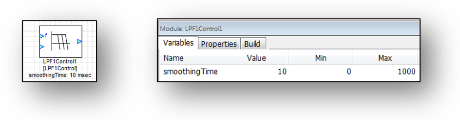
The LPF Control module is a time varying first order low pass with smoothly varying frequency based on the input pin.
Second Order Filter Control
The SOFControl filter is built upon the SecondOrderFilterSmoothed module. It has a fixed filterType which is specified on the inspector. Under module arguments, specify which of the filter design parameters should be obtained via input pins:
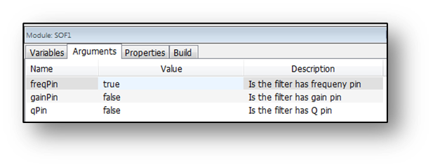
Parameters which aren’t specified by input pins are specified via the variables and properties tab. The SOFControl module uses deferred processing to compute the filter coefficients. That is, the design equation is not executed every block. Rather, when the control data on the input pin changes, the module sets a bit in its instance structure which causes the design function to be called from non-real-time code. This reduces the peak CPU load at the expense of having a slower update rate. In typical applications, the module will update every few 10s of milliseconds. If updating needs to happen more quickly, then use the FOFControl module or the ParamSet module coupled with a SecondOrderFilterSmoothed module.
A very common use of the SOFControl module is within a perceptual volume control. As the volume of the system is reduced, overall spectral balance should be maintained. Due to the sensitivity of the human auditory system, low frequencies and high frequencies appear to drop off more quickly than mid frequencies. Thus, to maintain the overall spectral balance, boost low and high frequencies as the volume level decreases. The VolumeControl module accomplishes this with a fixed boost table. For finer control over the boost, use a TableInterp module together with a SOFControl filter as shown below. The control signal “Volume” specifies the listening level and ranges from 0 (loud) to -80 (soft). The lookup tables convert the Volume setting into low frequency and high frequency boosts which are applied using the SOFControl module. The low frequency SOFControl module implements a peaking filter at 40 Hz and the gain is taken from the control pin. The high frequency SOFControl module implements a high shelf in which the gain is taken from the control pin.
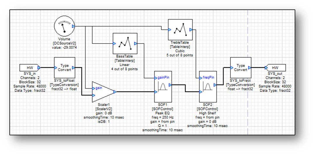
Example showing use of the SOFControl module in a table driven loudness control
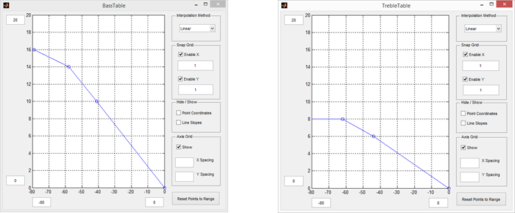
Lookup tables used in the table driven loudness control example. The left table converts the volume setting into a bass boost and the right table does the same for the high frequency adjustment.
Filters with Raw Coefficients
Audio Weaver contains several filter types which operate on raw coefficients. These filters are for expert users who understand DSP and know how to calculate the filter coefficients.
Note: MATLAB is often used by expert Audio Weaver users to compute coefficients and then update them in the block diagram.
There are two types of filters – Finite Impulse Response (FIR) and Infinite Impulse Response (IIR). Although Audio Weaver supports both types of filters, the majority of the filters used in audio applications are IIR due to their computational efficiency.
The most basic IIR filter is the Biquad and it is implemented with the difference equation:
𝑎0𝑦𝑛=𝑏0𝑥𝑛+𝑏1𝑥𝑛−1+𝑏2𝑥𝑛−2−𝑎1𝑦𝑛−1−𝑎2𝑦𝑛−2
There are 5 coefficients that the user must set: b0, b1, b2, a1, and a2 (a0 is always assumed to be 1). Audio Weaver does not check for stability and care must be used when computing the filter coefficients. There are several variants of Biquad filters. The simples – Biquad – has a single stage and implements the different equation shown above. BiquadCascade implements N stages of filtering with each channel using the same coefficients. BiquadNCascade implements N stages with each channel have its own set of coefficients. Finally, BiquadSmoothed implements a single Biquad stage with coefficient smoothing on a block-by-block basis.
 | FIR
| Time domain FIR filter Specify filter length in module properties |
 | Biquad
| Second order IIR filter. 5 filter coefficients are specified. No smoothing. |
 | BiquadCascade
| Multiple Biquad filters in series. The number of filters is specified in module properties. The same coefficients are used per channel. |
 | BiquadSmoothed
| Second order IIR filter. 5 filter coefficients are specified. Smoothed on a block-by-block basis |
 | BiquadNCascade
| Multiple Biquad filters in series. The number of filters is specified in module properties. Different coefficients are used per channel. |
 | FIR Sparse
| Sparse FIR filter in which most values are zero. Less convolution cycles than normal FIR |
 | FIR Sparse Reader
| Sparse FIR that connects to a delay state writer. Convolution is based on a pointer rather than a separate FIR buffer.
|
 | FIR Sparse Reader Fract16
| Like FIR Sparse Reader except half the memory. Data is converted to fract16 for computations and has a conversion for the output if necessary. |
High Precision Filters
Audio Weaver contains a variety of Biquad filters for equalizing audio. Some filters require raw coefficients (such as Biquad or BiquadCascade) while others contain built-in design equals (such as the SecondOrderFilter or ButterworthFilter). These filters are implemented using a Direct Form 2 (DF2) structure:
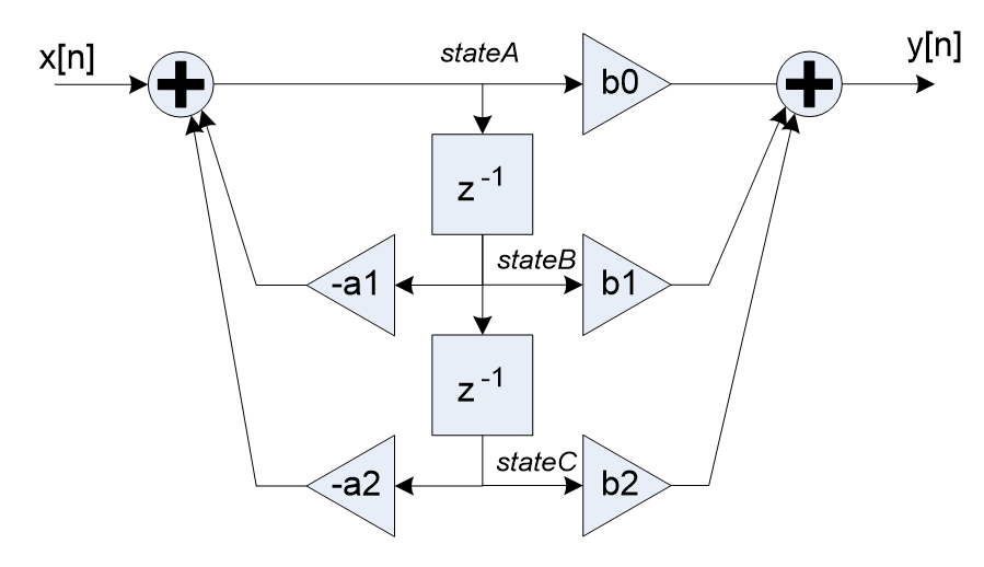
All Biquad filters including the DF2 have 5 coefficients. The advantage of the DF2 structure is that it requires only 2 state variables per filter as compared to 4 state variables for the DF1 structure.
These Biquad filters are implemented using floating-point arithmetic and are generally fine for most audio applications. Floating-point arithmetic, though, is not a panacea for all numerical issues and these filters can still suffer from quantization noise. The noise manifests itself as low-level noise correlated with the level of the input signal. Quantization noise is exacerbated by high sampling rates (96 kHz and above) and by having poles very close to the unit circle and this usually arises when making very low frequency EQ changes.
To solve these noise issues Audio Weaver includes a High Precision filter modules. These modules use floating-point input and output data and are compatible with the other floating-point modules. Internally the high precision filters use a proprietary DSP Concepts filter structure which significantly reduces quantization noise. The filters are also efficient with a typical Biquad requiring 7 MAC operations vs the 5 needed in a DF2 Biquad.
The High Precision modules are designed to be drop in replacements for the non-high precision filters. That way, numerical problems can be resolved by replacing the offending filter with its high precision version.
 | BiqudSmoothedHP | Smoothly varying Biquad |
 | ButterworthFilterHP | Butterworth lowpass, highpass, and allpass filters |
 | BiquadCascadeHP | Cascade of N Biquad stages |
 | GraphicEQBandHP | Single band of a graphic equalizer |
 | SOFControlHP | Controllable second order filter with design equations |
 | SOFCascadeHP | Cascade of second order filters each with design equations |
 | SecondOrderFilterHP | Single second order filter with design equations |
 | VolumeControlHP | Fletcher Munson volume control with loudness compensation |
The crossover filter module (XoverNway) is actually a subsystem consisting of multiple individual modules. The module properties give the option to construct the crossover using standard Biquads or high precision Biquads:
The graphic equalizer gives the option of using standard precision or high precision filters.
Here is an example of the benefits of the high precision filter. The system in the example has a peaking filter at 20 Hz with a gain of 6 dB and a Q of 2 and operates at a 48 kHz sample rate. The total harmonic distortion and noise (THD+N) for different input frequencies is plotted below. First for standard Biquad filters
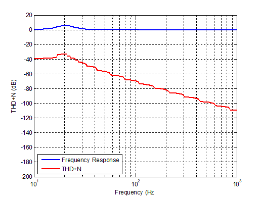
And now with a high precision filter, notice that the noise floor is reduced significantly – by up to 90 dB at low frequencies.
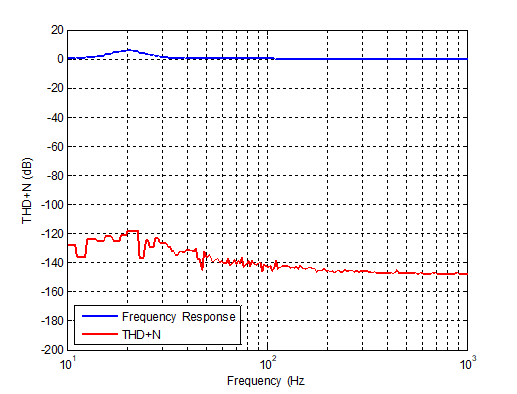
For the interested reader, this measurement is performed by passing sine waves of different frequencies through the filter. Apply a notch filter at the output which removes the sine wave and then measure the RMS energy in the residual. This residual energy equals the THD+N. The measurement is repeated for many different frequencies and the plot reflects the measured THD+N at each input frequency.
Common Filter Modules
The following filters are found as modules with no folder in the Filters directory. This is because they are the most common types of filters, which cover most general cases of filtering needs.
ButterworthFilter
This module implements lowpass, highpass, or allpass filters using a Butterworth design. The filters have a gain of 0 dB in the passband and are then monotonically decreasing in the stopband. The filter order is specified under module properties and ranges from 1st order (6dB/octave) to 10th order (60dB/octave). The filter order can only be changed in Design mode. Specify the filter type on the inspector (lowpass, highpass, or allpass) as well as the cutoff frequency, in Hz. Since these parameters are on the inspector, the filter type and cutoff frequency can be changed at run-time. Unfortunately, the ButterworthFilter does not have coefficient smoothing and there may be discontinuities when coefficients are updated.
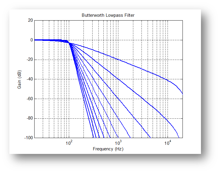
Butterworth lowpass filter frequency response as a function of filter order. The filter order goes from 1st order (least steep line) to 10th order (steepest line). The cutoff frequency is 100 Hz and the sample rate is 48 kHz
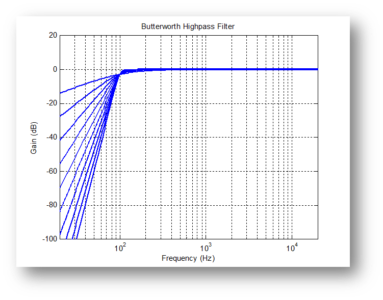
Butterworth high filter frequency response as a function of filter order. The filter order goes from 1st order (least steep line) to 10th order (steepest line). The cutoff frequency is 100 Hz and the sample rate is 48 kHz
SecondOrderFilterSmoothed
This module is the most frequently used filter among all of the Audio Weaver modules. It implements a 2nd order Biquad filter and includes design equations for 20 different filter types. The filter type and high-level design parameters (frequency, gain, and Q) can be changed at run-time using the inspector:
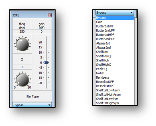
Depending on the filter type, some parameters are not used. See the table below for the filter types available and which control parameters are applicable.
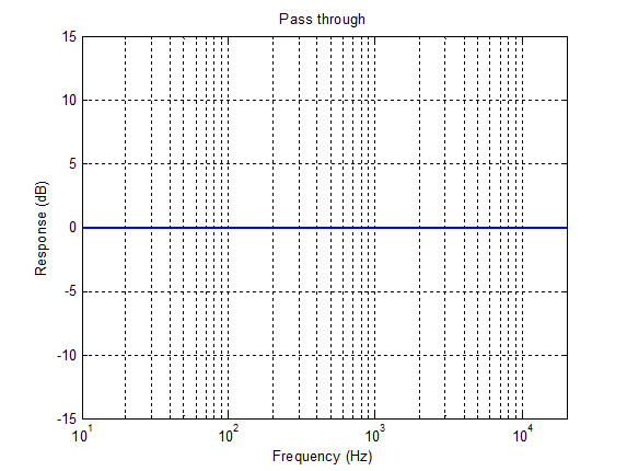
Pass Through filterType = 0
Applicable parameters: none.
Biquad coefficients are set to b0=1, b1=0, b2=0, a1=0, and a2=0. The filter runs and consumes processing but the output equals the input. |
 |
Gain filterType = 1
Applicable parameters: gain
A simple gain with coefficients set to b0=undb20(gain), b1=0, b2=0, a1=0, and a2=0 | 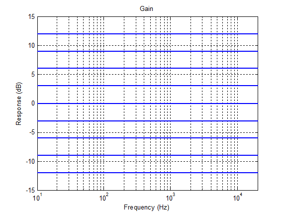 |
1st order Butterworth lowpass filter filterType = 2
Applicable parameters: freq | 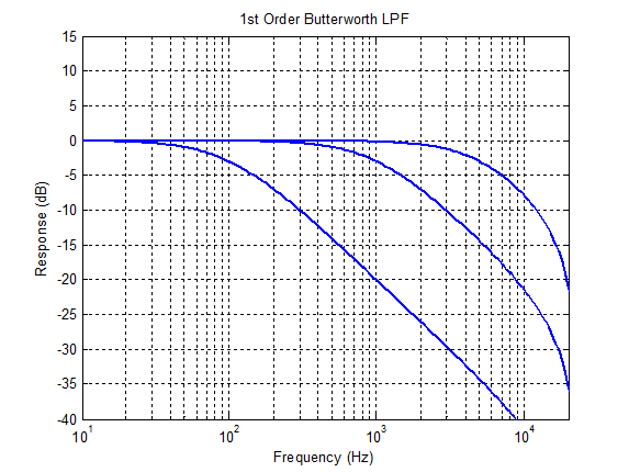 |
2nd order Butterworth lowpass filterType = 3
Applicable parameters: freq | 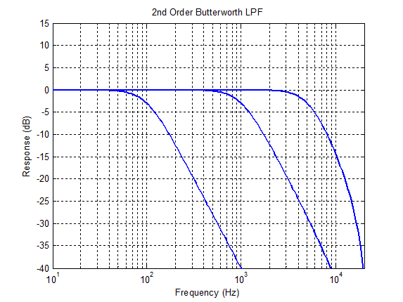 |
1st order Butterworth highpass filterType = 4
Applicable parameters: freq | 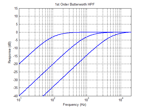 |
2nd order Butterworth highpass filterType = 5
Applicable parameters: freq | 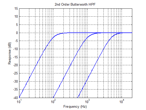 |
1st order allpass filterType = 6
Applicable parameters: freq |  |
2nd order allpass filterType = 7
Applicable parameters: freq and Q | 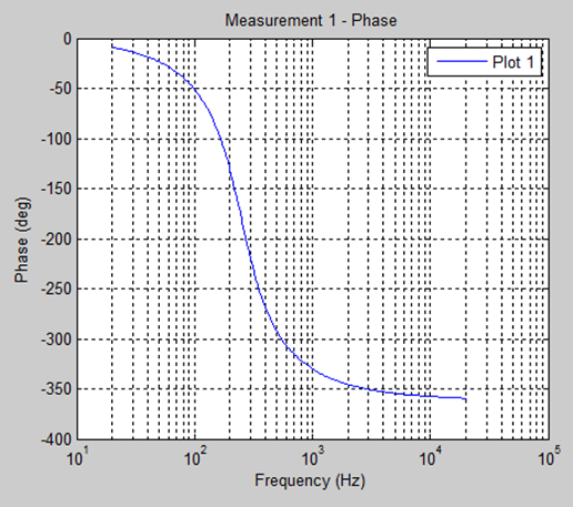 |
2nd order low shelf filterType = 8
Applicable parameters: freq and gain
Use as a low frequency tone control | 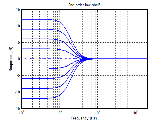 |
2nd order low shelf with Q filterType = 9
Applicable parameters: freq, gain, and Q | 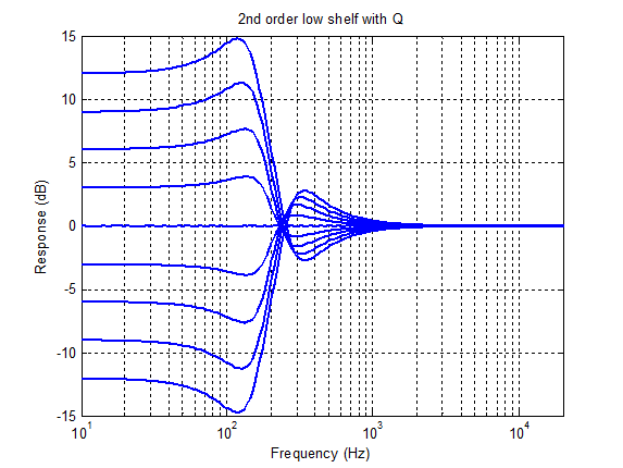 |
2nd order high shelf filterType = 10
Applicable parameters: freq and gain
Use as a high frequency tone control
| 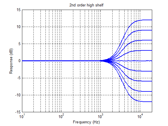 |
2nd order high shelf with Q filterType = 11
Applicable parameters: freq, gain, and Q | 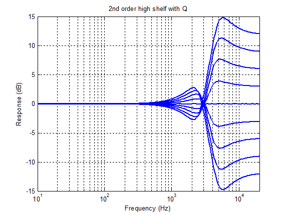 |
2nd order peaking / parametric filterType = 12
Applicable parameters: freq, gain, and Q
Commonly used for generic equalization since it has controllable frequency, gain, and Q settings. | 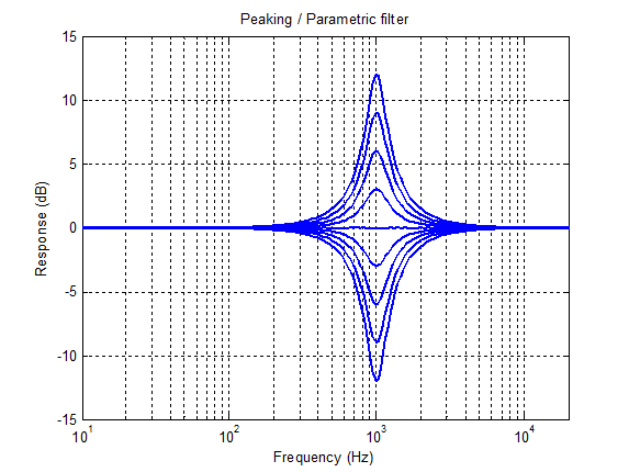 |
2nd order notch filterType = 13
Applicable parameters: freq and Q | 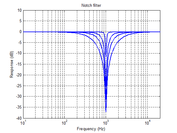 |
2nd order bandpass filter filterType = 14
Applicable parameters: freq and Q | 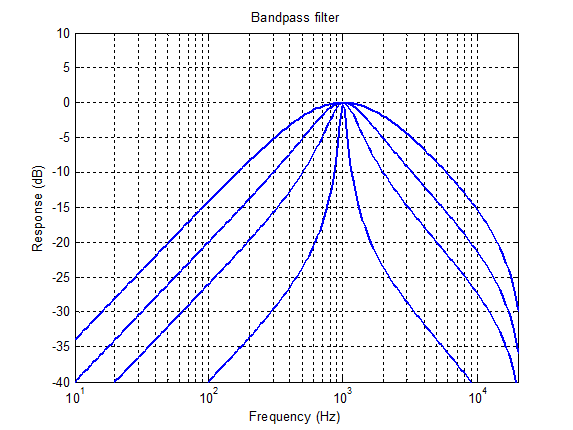 |
1st order Bessel lowpass filter filterType = 15
Applicable parameters: freq | 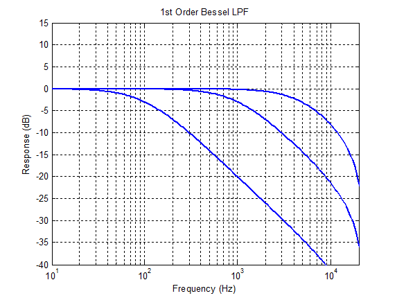 |
1st order Bessel highpass filter filterType = 16
Applicable parameters: freq | 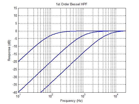 |
1st order asymmetrical low shelf filterType = 17
Applicable parameters: freq and gain | 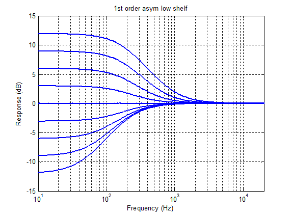 |
1st order asymmetrical high shelf filterType = 18
Applicable parameters: freq and gain | 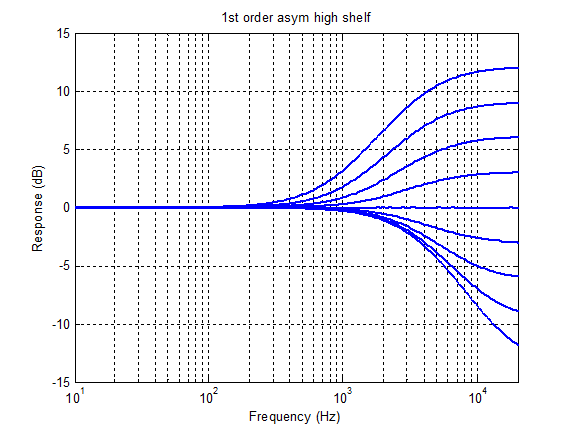 |
1st order symmetrical low shelf filterType = 19
Applicable parameters: freq and gain | 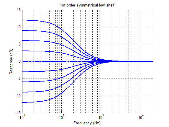 |
1st order symmetrical high shelf filterType = 20
Applicable parameters: freq and gain | 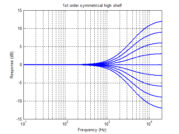 |
Note: The Butterworth filter from SecondOrderFilterSmoothed is the same as the ButterworthFilter module of equal filter order. However, SecondOrderFilterSmoothed only implements 1st and 2nd order Butterworth filters. Higher order Butterworth filters can only be implemented by the ButterworthFilter module.
The SecondOrderFilterSmoothed implementation of the first order Butterworth filter is more computationally efficient than the ButterworthFilter module.
Low/high shelf filter and low/high shelf filter Q are identical if Q is set to 0.707 (√0.5).
Second Order Filter Smoothed Cascade
This module contains several SecondOrderFilterSmoothed modules in series. This can be used to implement a more complicated EQ with only a single module. Under module properties, specify the number of stages of filtering. If the number of stages is set to 1, then this module is equivalent to the SecondOrderFilterSmoothed module. When there are multiple stages, the inspector expands as shown right:
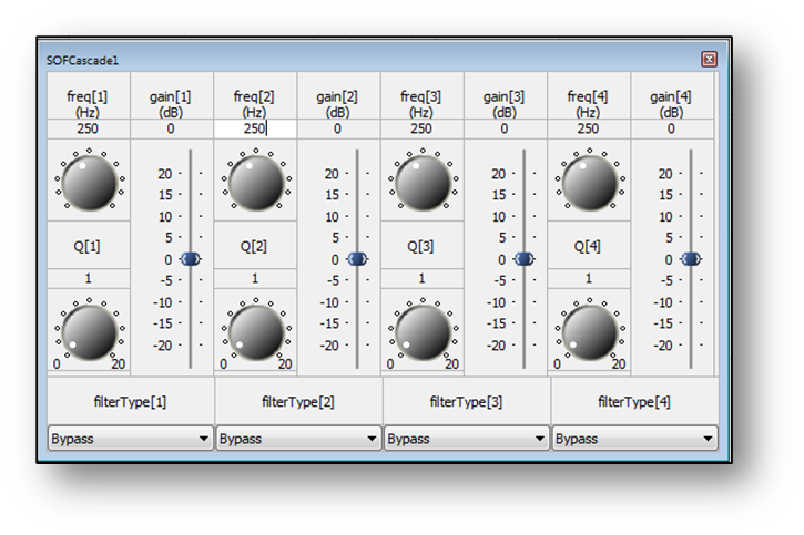
Table of Filter Modules
Category | Filter Type | Order | Usage Tip |
Adaptive | (FIR length) | signal to be learned' goes into reference pin. | |
Calculated Coeffs | Variable | set Rs for better band separation | |
Calculated Coeffs | Cascaded 2nd | change weighting with the dropdown variable. | |
Calculated Coeffs | Variable up to 10th | frequency will split into upper and lower bands | |
Calculated Coeffs | 1st | used typically by weighting formulas | |
Calculated Coeffs | Variable up to 12th | automatic frequency setting with module variables | |
Calculated Coeffs | Variable up to 12th | up to 12th order, useful. | |
Calculated Coeffs | 12th | +-90 degrees added to phase | |
Calculated Coeffs | 8th | turns white noise pink. Turns pink noise red. | |
Calculated Coeffs | 2nd | Cheap solution for handling "full spectrum" | |
Calculated Coeffs | Variable 2nd | Makes noise more 'blue' or 'pink' based on slope. | |
Controllable | 1st | immediate control | |
Controllable | 1st | immediate control | |
Controllable | 1st/2nd | delayed control | |
High Precision | Cascaded 2nd | High Precision, use for handling low freq, high SR, or sensitive ears. | |
High Precision | 2nd | (same) | |
High Precision | Variable up to 10th | (same) | |
High Precision | Variable up to 12th | (same) | |
High Precision | 1st/2nd | (same) | |
High Precision | Cascaded 1st/2nd | (same) | |
High Precision | 1st/2nd | (same) | |
Raw Coeffs | 2nd | clicks/pops with changes, this is for constant filter. | |
Raw Coeffs | Cascaded 2nd | same as above, higher order. | |
Raw Coeffs | 2nd | cascade with different filter responses. | |
Raw Coeffs | 2nd | smoothly varying, use for end-user control. | |
Raw Coeffs | (FIR length) | convolution FIR | |
Raw Coeffs | (FIR length) | FIR with mostly zeros, computationally efficient. | |
Raw Coeffs | (FIR length) | Hook to delay state writer, unique iterator feeds input for convolution | |
Raw Coeffs | (FIR length) | twice the memory efficiency as above. | |
Floating Modules | Variable up to 10th | Only odd allpasses are supported. Use SOF for even allpasses. | |
Floating Modules | 1st/2nd | 20 different filter types, varying orders. | |
Floating Modules | Cascaded 1st/2nd | same as above, but cascaded. |