Frequency Domain
This section contains the following pages:
Frequency Domain Math
- ComplexAngle
- ComplexConjugate
- ComplexConjugateFract32
- ComplexDivide
- ComplexMagnitude
- ComplexMagnitudeFract32
- ComplexMagnitudeSquared
- ComplexModulate
- ComplexMultiplierFract32
- ComplexMultiplierV2
- ComplexToPolar
- ComplexToRealImag
- ComplexToRealImagFract32
- PolarToComplex
- RealImagToComplex
- RealImagToComplexFract32
- Unwrap
General Information
Modules for processing signals in the frequency domain are found in the Frequency Domain folder. Frequency domain processing yields novels solutions to audio processing problems and may also lead to more efficient implementations. This section describes the main concepts behind frequency domain processing, then Filterbank Processing describes more sophisticated processing using weighted-overlap short-term Fourier transform filterbanks.
Complex Data Support
Audio Weaver natively supports complex data within wire buffers. The data is stored in an interleaved fashion:
real[0], imag[0], real[1], imag[1], real[2], etc
For multichannel data the interleaving of real and complex data happens at the lowest level. For example, interleaved stereo data is stored as:
L_real[0], L_imag[0], R_real[0], R_imag[0], L_real[1], L_imag[1], R_real[1], R_imag[1], etc.
Two modules are provided to convert between real and complex data
 | RealImagToComplex | Converts two real signals into complex data using one as the real part and the other as the imaginary part |
 | ComplexToRealImag | Converts a complex signal into separate real and imaginary components |
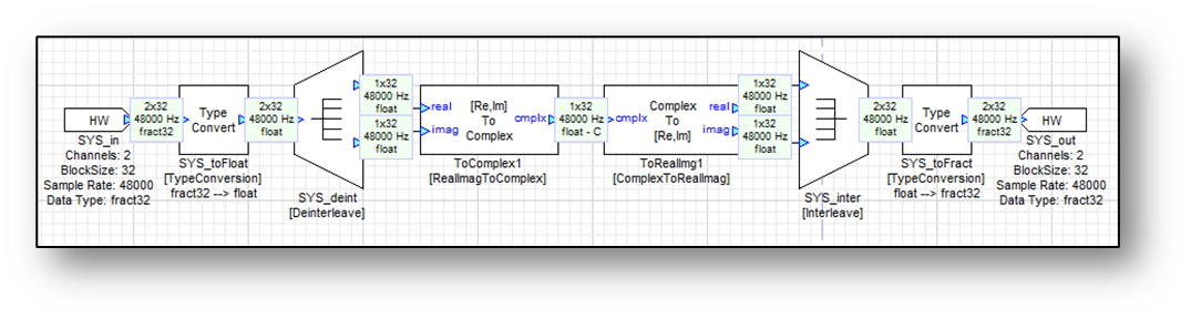
The system below essentially does nothing except convert two mono signals into complex and then back again. If view wire info is enabled, (“ViewàData type”) it will mark complex wires with a “C”.
Transform Modules
Audio Weaver provides 3 different transform modules for converting between the time and frequency domains.
 | Cfft | Complex FFT. Supports both forward and inverse transforms |
 | Fft
| Forward FFT of real data |
 | Ifft
| Inverse FFT yielding real data |
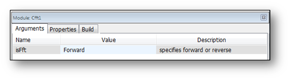
The complex FFT takes a complex N-point input and generates a complex N-point output. The module is configured on the module properties as either a forward or inverse transform.
The Fft and Ifft modules are designed to operate on real signals. The Fft modules takes an N-point real input and generates an N/2+1 point complex output. The output signal contains frequency samples from DC ( ) all the way up to and including the Nyquist frequency ( ). A property of the real FFT is that the samples at DC and Nyquist contain real data only and the imaginary components are guaranteed to be zero. These samples are still stored as complex values but the imaginary component is zero. The output of the real FFT will therefore consist of the samples:
X[0] real
X[1] complex
X[2] complex
…
X[N/2-1] complex
X[N/2] real
The Ifft takes N/2+1 complex samples and returns a real N-point sequence. The Ifft ignores the imaginary component of the DC and Nyquist samples.
Windowing
Before an FFT is computed the signal is typically windowed to prevent edge effects from influencing the results. There are 3 modules which perform windowing.
 | Window | Simple window |
 | WindowOverlap
| Window with overlapping |
 | WindowAlias
| Windowing followed by time aliasing |
The windowing modules are for advanced users who use MATLAB to compute window coefficients.
The Window module can compute a large number of different window functions. Under module properties, specify the length of the window to apply. Then on the inspector, specify the starting and ending indexes of the window as well as the window type and an optional amplitude.
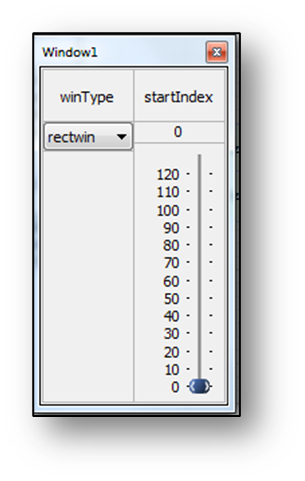
Allowing the ability to change the starting and ending indexes of the window is more flexibility than is usually needed.
The WindowOverlap module has an internal FIFO that buffers up data into overlapping blocks. For example, a 64-sample input block size with a 50% overlap turns into 128 sample blocks, to be windowed. Essentially, the WindowOverlap module contains a Rebuffer module combined with a Window module. The module has an internal array of window coefficients. This array is initialized to a Hamming window (raised cosine) at instantiation time. To change the window coefficients use the Matlab scripts.
The WindowAlias module applies a window followed by time aliasing the sequence to a shorter length. This module is used in the analysis back of short-term Fourier transform based filterbanks.
 | OverlapAdd | Reduces block size by overlapping blocks |
The OverlapAdd module performs the opposite of the Rebuffer module. The module has a large input block size and a smaller output block size. The module contains an internal buffer equal to the input block size. The module takes the input data, adds it to the internal buffer, and then shifts out one block of output data. The data in the internal buffer is also left shifted and the leading samples are filled with zeros. The OverlapAdd module finds use in fast convolution algorithms.
 | RepWinOverlap | Replicates data, applies a window, and then performs overlap add |
The RepWinOverlap module is for advanced users building synthesis filterbanks. The module replicates a signal N times, applies a window, and then performs overlap add.
 | ZeroPad | Adds zeros at the end of a buffer |
The ZeroPad module inserts zeros at the end of a signal. Specify the length of the output buffer under module properties. If the output is longer than the input then the signal is zero padded. If the output is shorter than the input then the signal is truncated.
Complex Math
The frequency domain modules have a large number of modules which operate on complex data. The modules here are listed without detailed explanations because the underlying functions are basic and easily understood.
 | ComplexAngle | Computes atan2 of complex data |
 | ComplexConjugate | Conjugates data by negating the imaginary component |
 | ComplexMagnitude |  |
 | ComplexMagSquared |  |
 | ComplexModulate | Multiplies by 𝑒𝑗𝜔𝑘 |
 | ComplexMultiplier | Complex x Complex, or Real x Complex |
 | ComplexToPolar | Converts to Polar (angle and magnitude) |
 | PolarToComplex | Converts from Polar to Real/Imag |
The modules listed above operate on complex data only. A few of the other Audio Weaver modules found outside the Frequency Domain folder are also able to operate on complex data type:
Module | Operation |
|---|---|
BlockConcatenate | Combines blocks of complex data |
BlockDelay | Delays by multiples of the block size |
BlockExtract | Extracts a portion of the complex data |
BlockFlip | Frequency flips data |
Deinterleave | Pulls apart multichannel complex signals into individual mono complex signals |
Demultiplexor | Outputs complex data to one output pin; zeros the rest |
Interleave | Combines multiple mono complex signals into a single multichannel complex signal |
Multiplexor | Selects one of N complex signals |
ShiftSamples | Left or right shifts complex signals |
Adder | Adds two complex signals |
ClipAsym | Clips the real and imaginary components |
Invert | Multiplies by + or -1. Set smoothingTime = 0. |
Mixer | Mixers together complex signals |
MixerDense | -Mixers together complex signals |
MuteSmoothed | Multiplies by +1 or 0. Set smoothingTime = 0. |
ScaleOffset | Scale both the real and imaginary components and adds an offset |
ScalerDB | dB gain without smoothing |
Scaler | Linear gain without smoothing |
Subtract | Subtracts two complex signals |
SumDiff | Adds and subtracts complex signals |
WhiteNoise | Generates uncorrelated noise in both real and imaginary components |
ScalerDBControl | dB gain with gain value taken from a control pin. Set smoothingTime = |
ScalerControl | Linear gain with the gain value taken from a control pin. Set smoothingTime = 0 |
FilterBank Processing
Introduction
This Section describes the filterbank blocks. The blocks are based on a weighted overlap-add (WOLA) design and are applicable to a wide range of audio processing tasks. The document first describes how the blocks work from an end user’s point of view. It then describes the theory behind the filterbanks and how they lead to efficiency during runtime.
Using WOLA and sub-band Blocks
The WOLA filterbank blocks are part of the DSPC Concepts IP Folder. The Frequency Domain contains the key set of Audio Weaver modules which are used for performing frequency domain computations. There are blocks for FFTs, windowing, complex operations, etc. Frequency domain operations often involve filterbanks, and Audio Weaver also includes modules for implementing entire weighted overlap-add filterbanks. There are separate modules for the forward filterbank (the analysis bank) and the inverse filterbank (the synthesis bank).
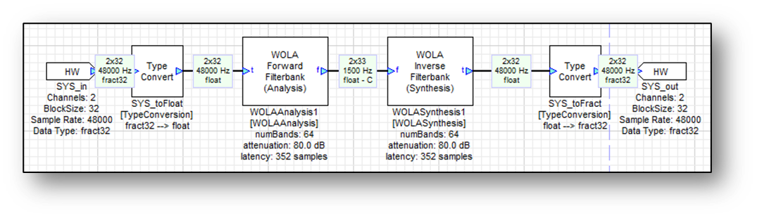
The blocks are called “WOLA Analysis” and “WOLA Synthesis”. When dragged out, they will appear as follows in the layout:
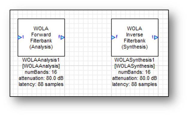
The input to the WOLA Analysis bank is real time domain data and the output is complex frequency domain data. Similarly, the input to the WOLA Synthesis bank is complex frequency domain data and the output is real time domain data. When configuring the filterbanks using Module Name and Arguments, the FFT size (K) and the stopband attenuation between subbands is specified. This holds for both the analysis and the synthesis banks. Under module name and arguments, this would show:
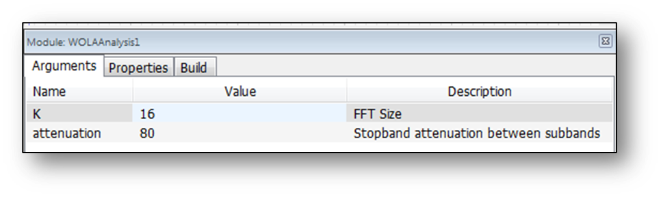
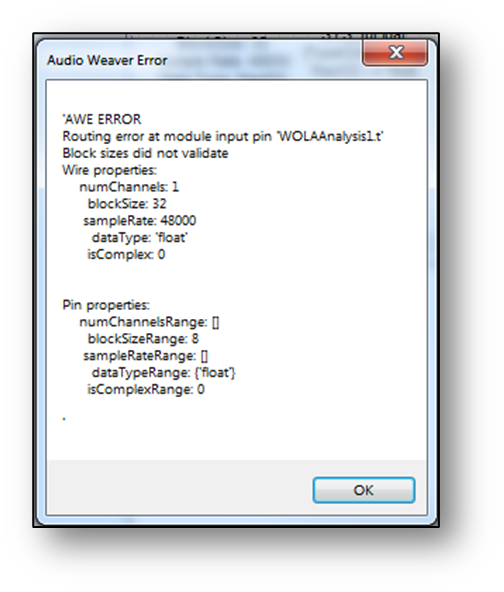
The FFT specifies the number of frequency domain “bins” and the input (and output) block size is always ½ of the FFT size. For example, if using a 32 sample block size will only work with an FFT size K = 64. Manually set this on both the analysis and the synthesis filterbanks. This will error out if improperly specified:
The attenuation relates to the separation between outputs of the filterbank, in dB, and will be described in more detail later in the guide. A “safe” value to use is somewhere in the range from 40 to 80 dB. When combining analysis and synthesis filterbanks, ensure that the same value of attenuation is used throughout.
Assuming a block size of 32, set the FFT size K = 64. Making connections between blocks and then showing wire sizes:
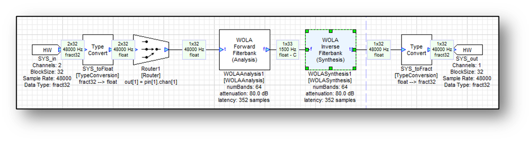
Note that the output of the filterbank contains 33 complex samples rather than 64. This is because the filterbank modules use real FFTs and as a result discard the redundant conjugate symmetric data. Only K/2+1 bins are kept, which in this case equals 33. The bins have the following properties:
Bin k=0. Real data.
Bin k=1. Complex data.
Bin k=2. Complex data.
…
Bin k=31. Complex data
Bin k=32. Real data
The first and last bins have real data; this is a property of the FFT and results from the fact that the input data is real. Audio Weaver stores the output of the FFT as 33 complex values with the imaginary parts of bins k=0 and k=32 set to zero.
The filterbanks accept any number of channels of input data, but it is not a typical scenario in Audio Weaver.
Note: Although the analysis and synthesis filterbanks accept any number of channels, most modules in the Frequency Domain folder only operate on mono signals. It is recommended to design systems with mono frequency domain data for greatest flexibility.
The text below the filterbank modules also shows the latency through the filterbanks, in samples. The latency is the combined latency through the analysis and synthesis filterbanks given the current values of K and attenuation. Increasing K or increasing the attenuation increases the latency through the filterbanks. use the displayed latency to time align other signals in the system. For example, to check the reconstruction properties of the filterbanks, compensate using a sample delay module:
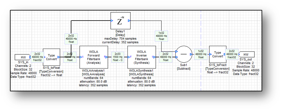
The output of the WOLA synthesis bank equals the input of the analysis bank but delayed by 352 samples. In the example above, this latency is compensated with a delay, so the output of the subtract module is essentially zero.
This example shows the meter module with a residual difference at around -80 dB. The filterbanks are not perfect reconstruction but introduce a small amount of aliasing noise. The level of aliasing noise is directly related to the attenuation setting of the filterbanks.
The frequency domain outputs of the analysis filterbank represent the outputs of a series of bandpass filters. There are K filters and the spacing between bins is 2π/K radians, or if the sample rate of the system is SR, then the spacing between bins is SR/K Hz. For example, if the sample rate of the system is 48 kHz and K=64, then the spacing between bins is 750 Hz. The first bin (with real data) is centered at 0 Hz. The next bin is centered at 750 Hz, and so on. The last bin (with real data) is centered at 24 kHz.
The filterbanks also contain built in decimation. The outputs of the analysis bank represent the decimated outputs of bandpass filters. The decimation factor equals the block size, that is, K/2. Continuing the example from above, the sample rate of the system is 48 kHz and the block size is 32 samples. Thus, the sample rate of the frequency domain subbands is 1500 Hz. see this by showing the sample rate on the wires.
Theory
This section describes more of the mathematical theory behind the filterbanks. The design of the filterbanks was based primarily on chapter 7 of the book Multirate Digital Signal Processing by Crochiere and Rabiner. This is an excellent and very readable introduction to the subject of filterbanks. Our description follows the derivation found in this book.A classical filterbank uses a time domain window function followed by an FFT as shown below:
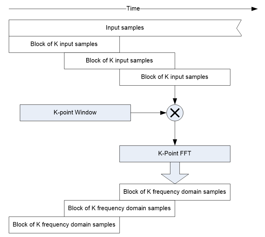
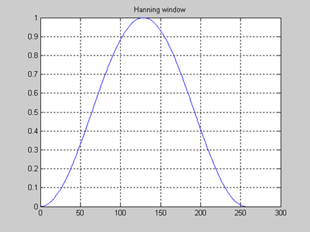
The length of the FFT equals the length of the window function. In many cases, the window function is a raised cosine, or Hanning window:
The input blocks of the filterbank are overlapped in time. There are many ways to describe the amount of overlapping. The terminology “50% overlap” indicates that from FFT to FFT, K/2 new input samples are made. If there is “75% overlap” then there are K/4 new samples for each FFT computed. In this discussion, the phrase “block size” is used to describe how many new samples arrive each time. This approach is also referred to as a short-term Fourier transform (STFT).
There are two different ways of looking at the output of the STFT analysis bank. On is to segment the input signal into blocks which are windowed and then FFT’ed. The output of the analysis bank thus corresponds to frequency spectra. On the other hand, a careful study of the analysis bank shows that it is in effect implementing a set of parallel bandpass filters as shown below.
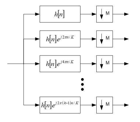
Analysis filterbank implementation as a parallel set of bandpass filters and decimators.
The input signal is filtered and then decimated by the block size M. The filters are all related by the mathematical expression
ℎ𝑘[𝑛]=ℎ0[𝑛]𝑒𝑗2𝜋𝑘𝑛/𝐾
where is the prototype lowpass filter and all other filters are related to the prototype filter by complex modulation. In the frequency domain, the filters are shifted versions of the prototype filter
𝐻𝑘(𝜔)=𝐻0(𝜔−2𝜋𝑘/𝐾)
For example, if a Hanning window is used as the prototype filter,
ℎ[𝑛]=121−cos(2𝜋𝑛𝐾)−1
then the frequency response for K = 32 is
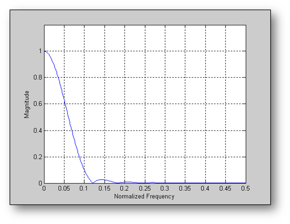
Frequency response of a 32-point Hanning window. The graph shows normalized frequencies in the range 0 to 1.0 which corresponds to 0 to radians/sample.
Subsequent bins are spaced by (or when viewed as normalized frequencies) and the first 4 bins are shown below:
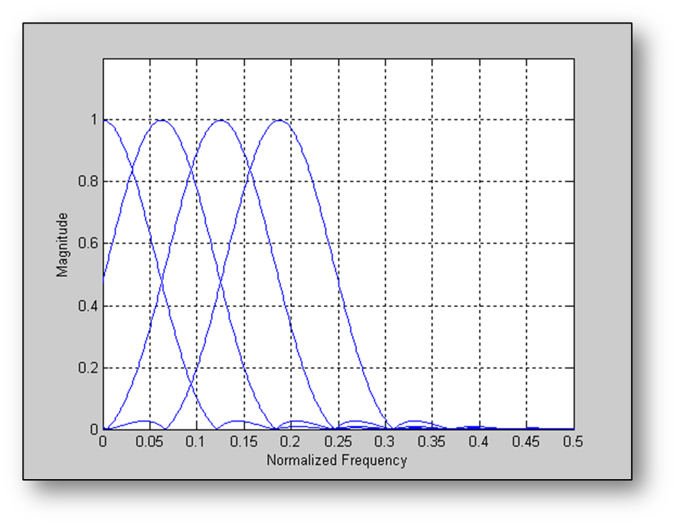
Note: The prototype filter is quite wide in the frequency domain and there is significant overlap between neighboring bins. Not only does bin k overlap with bin k+1, but also with k+2 and k+3. If a decimation factor of 16 is picked, then aliasing will start at normalized frequency of 1/16 as shown below. The prototype filter has only attenuated the signal by 0.5 and severe aliasing will occur.
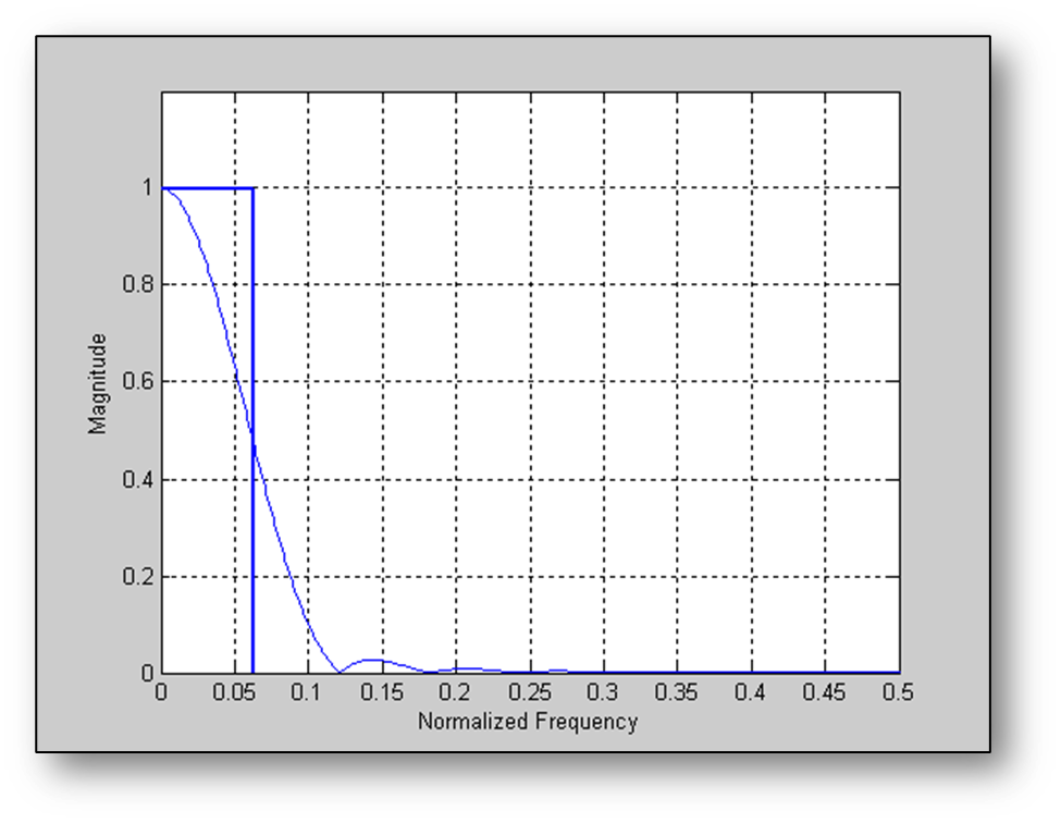
Frequency response of a 32-point Hanning window overlayed with a rectangle indicating where aliasing would occur if the filter output is decimated by a factor of 16
If the decimation factor is changed to 8, then aliasing begins at a normalized frequency of 1/8 SR and the filter has attenuated the signal. However, with a decimation factor of 8 the 32 sample Hanning window only advances 8 samples each time and this corresponds to an overlap factor of 75%.
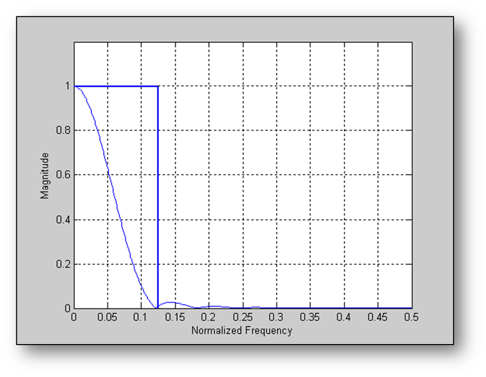
This time the rectangle indicates where aliasing occurs for a decimation factor of 4.
Is there a way to achieve high decimation while at the same time avoiding aliasing? This brings up the weighted overlap-add filterbank (WOLA). The block based derivation from Crochiere and Rabiner avoids aliasing while supplying high decimation. The analysis filterbank is implemented as shown:
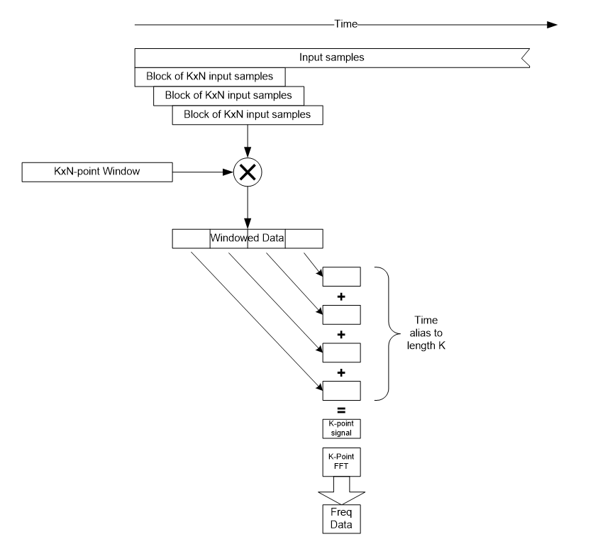
The main difference is that the prototype filter is N times longer and that after multiplying the input signal, the output is time aliased to the FFT length. Time aliasing is a standard property of the FFT. Suppose an input signal is given: 𝑟[𝑛] of length . Time alias this to a shorter signal of length
𝑥[𝑛]=𝑝=0𝑁−1𝑟[𝑛+𝑝𝐾]
The FFT 𝑥[𝑘] of 𝑥[𝑛] is related to the FFT R[𝑘] of ??[𝑛] by subsampling
𝑋[𝑘]=R[𝑘N]
That is, 𝑋[𝑘] contains samples of R[𝑘] spaced by N bins.
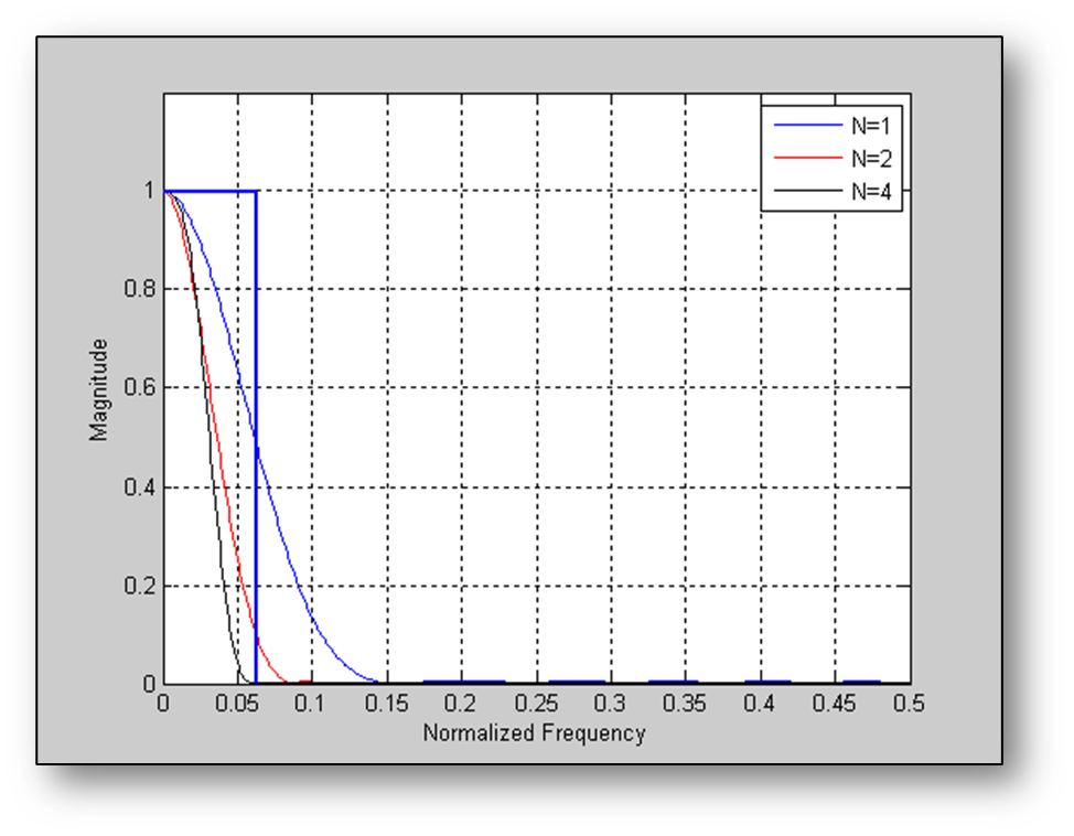
The advantage of using a longer prototype filter is that it allows us to get better frequency separation between bands. Consider the designs shown below with N=1, N=2, and N=4. The filters get progressively sharper in frequency and for N=4, the passband of the filter falls within the rectangle indicating the aliasing region for a decimation factor of 16. Thus a high decimation factor is achieved while avoiding high amounts of aliasing.
Now let’s plot the frequency response of the first 4 filters in the filterbank assuming an FFT size of 32 samples, a window length of 128 samples, and a decimation factor of 16.
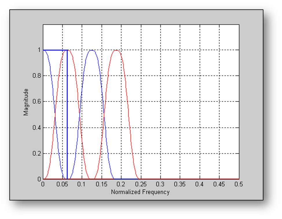
First 3 subband filters for the WOLA filterbank with K=32, N=4, and a decimation factor of 16.
When N is increased to a very high number to achieve a decimation factor of 32, the result is a critically sampled filterbank with no net increase in data. This limit can be approaced, but never achieved in practice. With realizable filters, a filter will always overlap its immediate neighbors. In Audio Weaver, a decimation factor of K/2 is used and the filterbanks are oversampled by a factor of 2. There is a net doubling of the data rate, but this is important because it decouples the subbands and allows them to be modified without introducing further aliasing distortion.
Recent theory of filterbanks has been focused on critically sampled filterbanks. These filterbanks find use in audio compression and since the goal in compression is to reduce the overall data rate, it is important not to oversample and introduce more data in the subband representation. However, the operations performed on subbands in audio codecs are very gentle compared to what is possible with our WOLA filterbanks. In audio compression, the goal is for the output to equal the input. In Audio Weaver processing systems, the focus is to be able to make gross changes to the subbands without introducing objectionable aliasing artifacts. This requires a fundamentally different approach. Furthermore, if the algo calls for a frame overlap add and overlap save convolution in a filterbank framework, oversampling is needed. In general, in order to perform subband modifications of audio signals without introducing objectionable aliasing distortion, some amount of oversampling is required.
Aliasing Performance of the WOLA Filterbanks
As noted above, the filters in the filterbanks are not ideal and introduce some amount of aliasing. The amount of aliasing depends upon the stopband attenuation used in the design of the filters. This section provides details on the amplitude of this aliasing noise. To test this, use the system shown below:
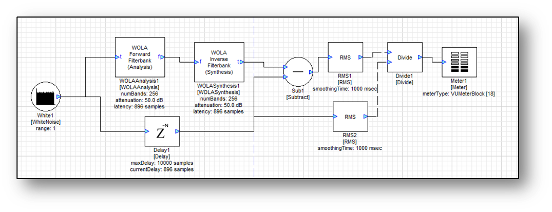
Analysis and synthesis filterbanks are placed back-to-back. The input is white noise, the output is subtraction of the inputs while compensating for the delay through the filterbanks. Comparing the energy at the input to the energy of the residual noise provides an indication of the level of the aliasing components. The following table shows the aliasing level and latency as a factor of the stopband attenuation of the prototype low pass filter. In the test, an FFT size of 256 samples was used with a resulting blockSize of 128 samples.
Stopband Attenuation (dB) | Measured Aliasing Noise (dB) | Latency (samples) | Latency (blocks) |
|---|---|---|---|
30 | -28 | 384 | 3 |
40 | -39 | 640 | 5 |
50 | -50 | 896 | 7 |
60 | -61 | 1152 | 9 |
70 | -61 | 1152 | 9 |
80 | -78 | 1408 | 11 |
90 | -87 | 1664 | 13 |
Keep in mind that the aliasing components are linearly related to the input signals. That is, reducing the level of the input signal by 20 dB results in the level of the aliasing components dropping by 20 dB. Thus, the aliasing level is more similar to a signal to noise ratio (SNR) rather than total harmonic distortion.
Subband Signal Manipulation
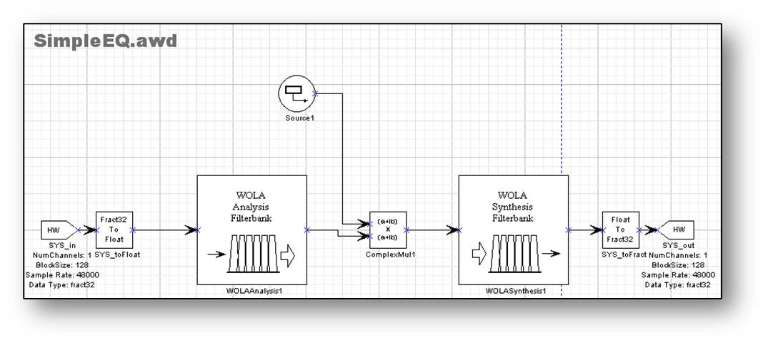
Part of the beauty of these filterbanks is that it is possible to manipulate the signals in the subband domain. For example, if scaling the subband signals as shown below, the result will be an equalizer with linearly spaced frequency bins.
Another nice property of the WOLA filterbanks is that they have built in smoothing. That is, making an instantaneous gain change to one of the subband signals then the net effect at the output will be smooth. This is because the synthesis bank has built in low pass filters in each subband and these smooth out discontinuities.
The FIR filter example can be taken further. The example above had only a single gain within each subband. What if the goal is to have more frequency resolution? Place FIR filters into each subband. A longer FIR filter would provide more resolution within that particular frequency band. Consider the following example. A filterbank has an FFT size of 64 samples and is operating with a decimation factor of 32. If the input is 48 kHz then each subband has a sample rate of 1.5 kHz. If an FIR filter of length 500 samples is placed in the DC subband (bin k=0), then this yields an effective frequency resolution of 3 Hz within this band. The amount of computation needed to implement this filter is approximately 1500 x 500 = 0.75 MIPs. High resolution is needed in audio applications at low frequencies. For higher frequencies, reduce the lengths of the FIR filters and achieve something close to “log frequency resolution”. By proper design of the subband filters, designing phase response becomes simple.
Any of the Frequency Domain modules which operate on complex data operate in the subband domain. Audio Weaver also provides a special set of “Subband Processing” modules that start with the “Sb” prefix. These modules replicate some of the standard time domain modules but the operations occur separately in each subband.
 | SbAttackRelease | Attack and release envelope follower (real data only) |
 | SbDerivative | Derivative (real data only) |
 | SbComplexFIR | Complex FIR filter |
 | SbNLMS | Normalized LMS adaptive filter |
 | SbSmooth | Performs smoothing across subbands (real data only) |
 | SbRMS | RMS with settable time constant (real data only) |
 | SbSOF | Second order filter (real data only) |
 | SbSplitter | Subdivides the spectrum into overlapping regions. Similar to a crossover |
Synthesis Filterbank
The synthesis filterbank takes the subband signals and reconstructs a time domain output. Error! Reference source not found.Remember that the analysis filterbank can be considered to be a parallel set of bandpass filters and decimators. The synthesis filterbank uses a the inverse of this with upsamplers, filters, and adders. The upsamplers take the decimated subband signals and return them to the original sampling rate by inserting M-1 zeros between each sample value. In the frequency domain, upsampling creates copies of the input spectrum at multiples of and the filters remove the high frequency copies.
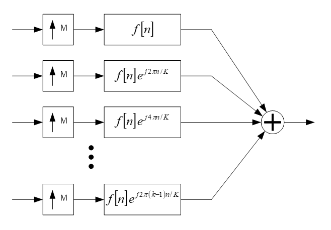
Synthesis filterbank implementation using upsamplers and bandpass filters.
For efficiency, the synthesis filterbank is implemented using an inverse FFT and periodic replication. As in the analysis filterbank, the window function f[n] corresponds to the impulse response of the prototype lowpass filter used in subband k=0.
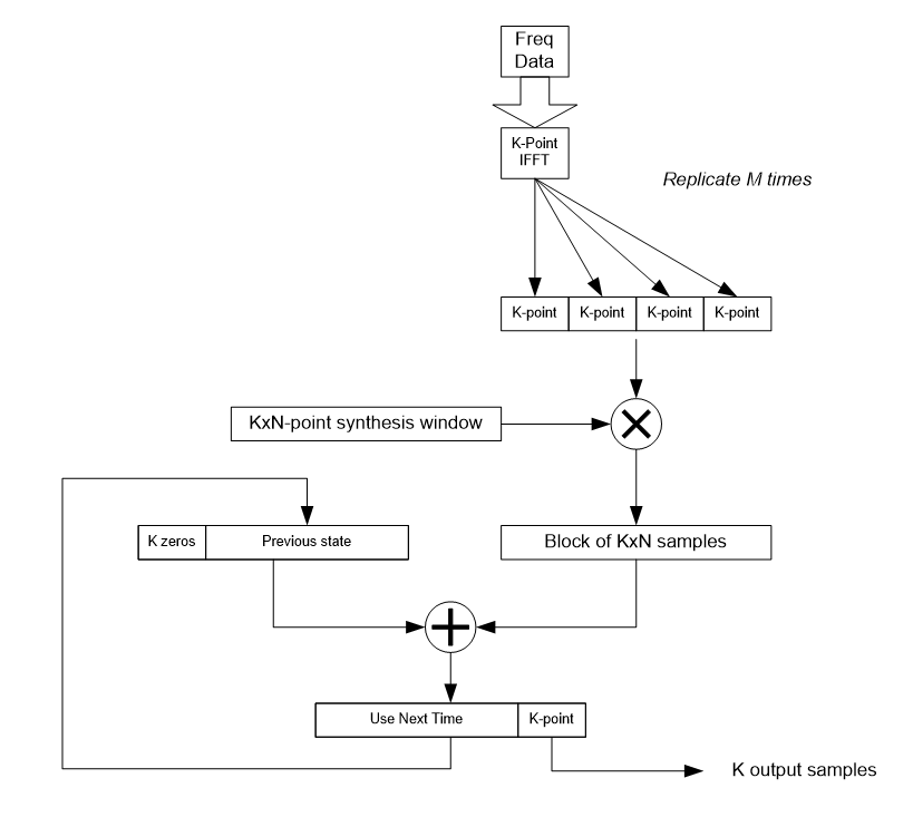
Synthesis bank implemented using an inverse FFT followed by windowing and overlapping.